pytorch日积月累4-梯度与自动求导
1.深度学习的核心——梯度
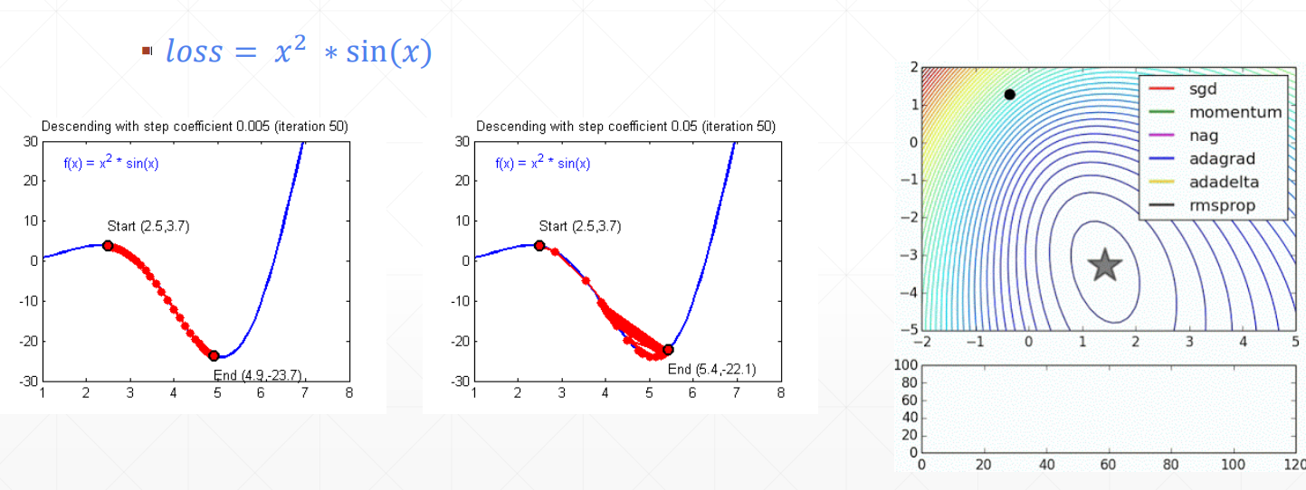
learnrate:学习率,迭代速度的限制因素。
设置不同的梯度下降的求解器
1 | import numpy as np |
2.随机梯度
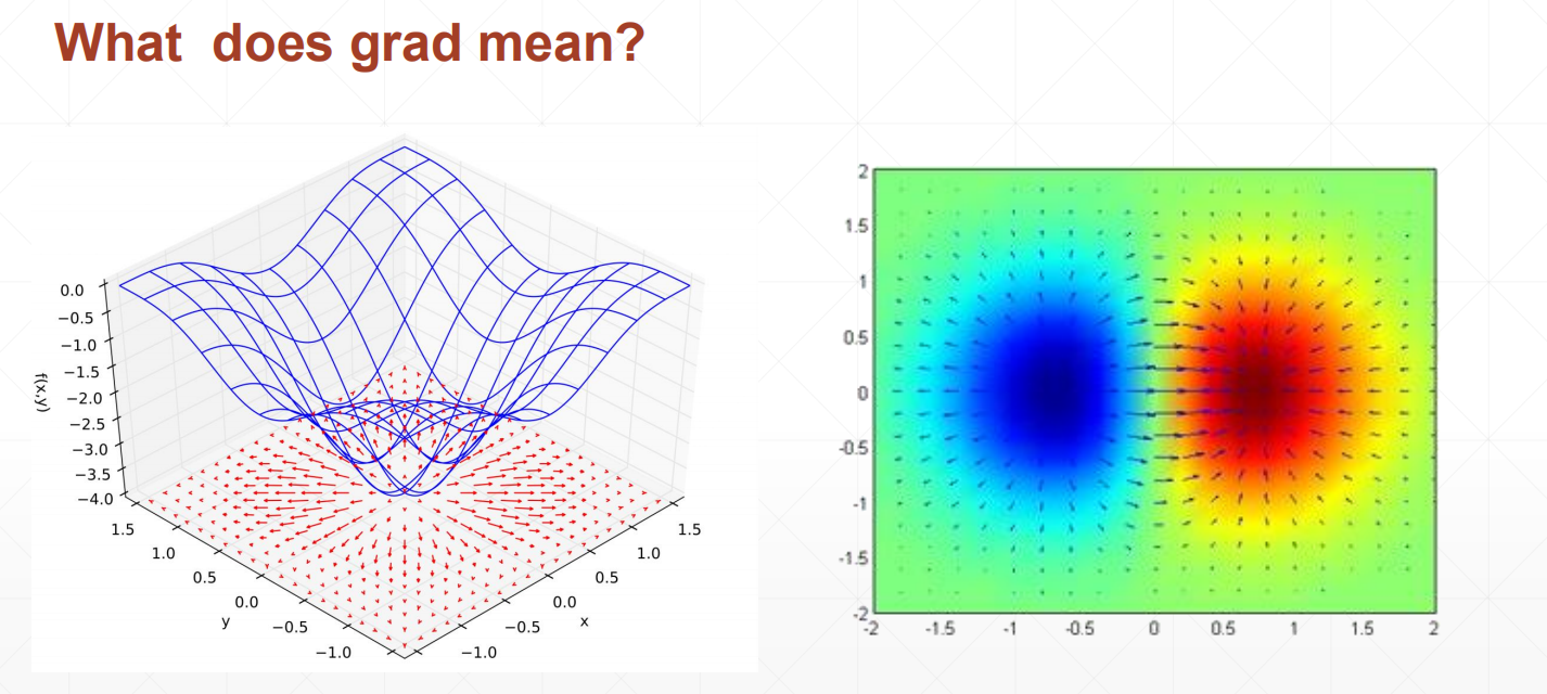
2.1什么是梯度
Optimizer Performance
▪ initialization status(初始值)
▪ learning rate(学习率)
▪ momentum(动量,惯性)
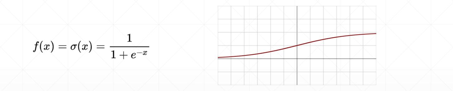
2.2激活函数及其梯度
激活函数:
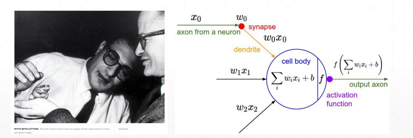
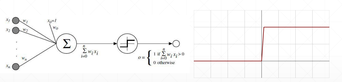
最简单的激活函数:
Sigmoid / Logistic函数——光滑可导
1 | import torch |
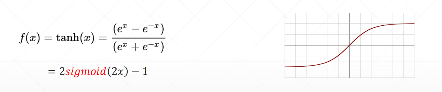
Tanh——RNN中用的较多
1 | import torch |
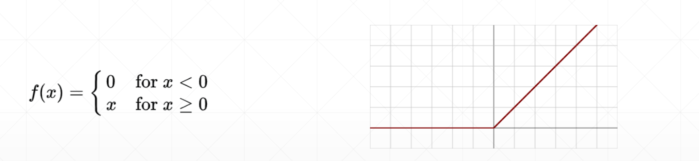
Rectified Linear Unit——RELU——非线性激活函数
1 | from torch.nn import functional as F |
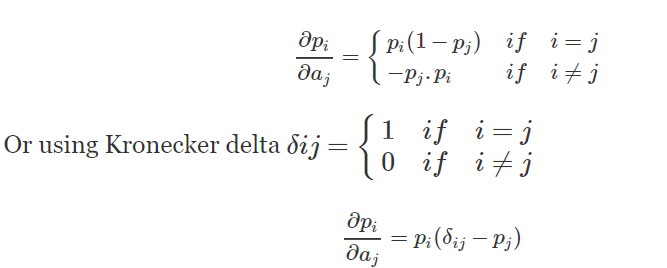
2.3LOSS及其梯度
Mean Squared Error(MSE)
Derivative
torch.autograd.grad(loss, [w1, w2,…])——->[w1 grad, w2 grad…]loss.backward()—->w1.grad w2.grad
1 | x=torch.ones(1) |
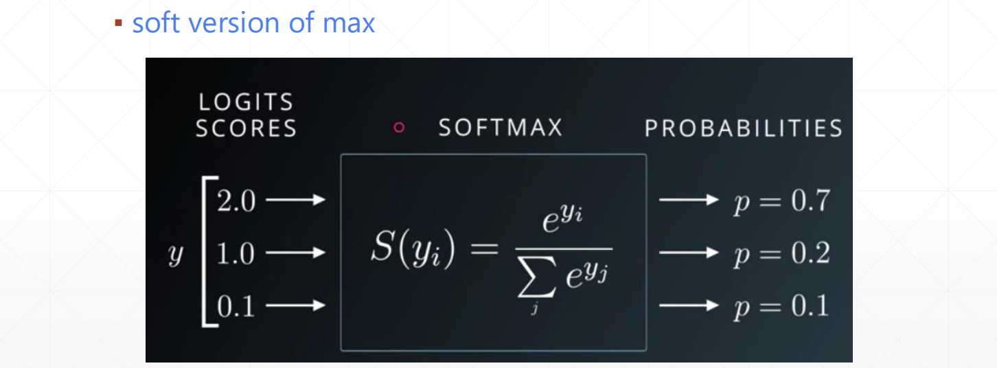
softmax
2.4利用pytorch实现线性回归
1 | import torch |
3.自动求导
3.1torch.autograd
torch.autograd.backward- 功能:自动求取梯度
- 函数说明如下:
1 | #第一个常用的函数 |
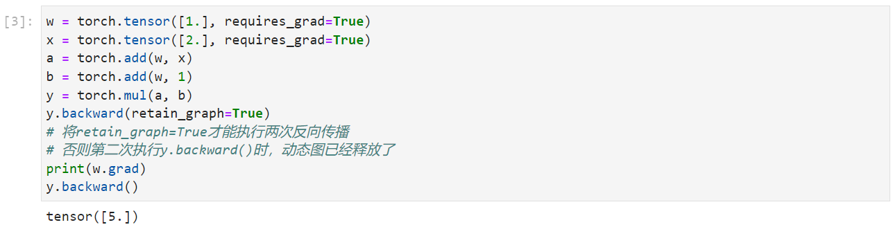
使用反向传播计算梯度:
retain_graph=True用于保存动态图
1 | w = torch.tensor([1.], requires_grad=True) |
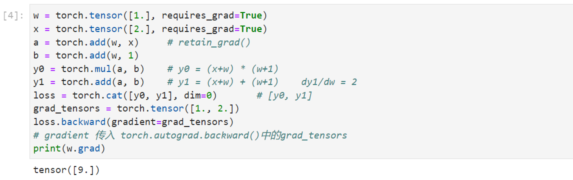
gradient=grad_tensors用于多个梯度之间的权重计算
1 | w = torch.tensor([1.], requires_grad=True) |
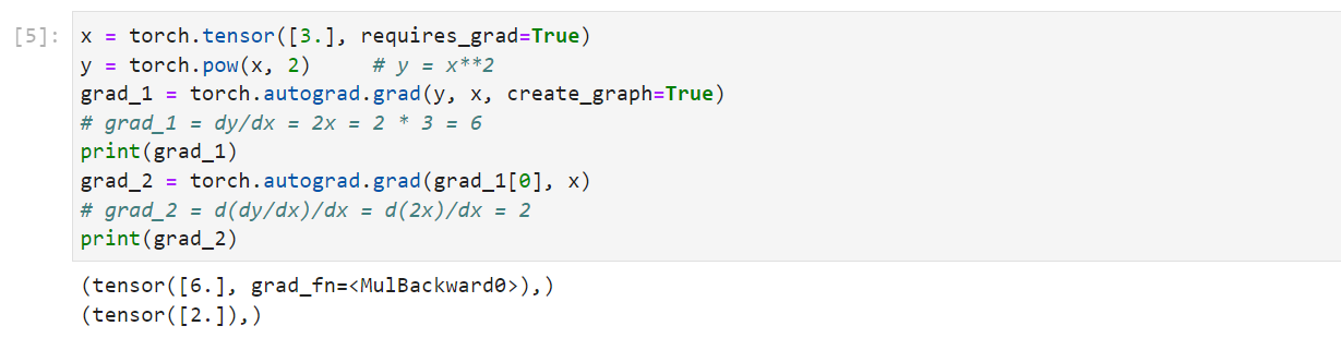
torch.autograd.grad- 功能:求取梯度
- 函数说明如下:
1 | torch.autograd.grad(outputs,#用于求导的张量 |
1 | x = torch.tensor([3.], requires_grad=True) |
autograd小贴士:
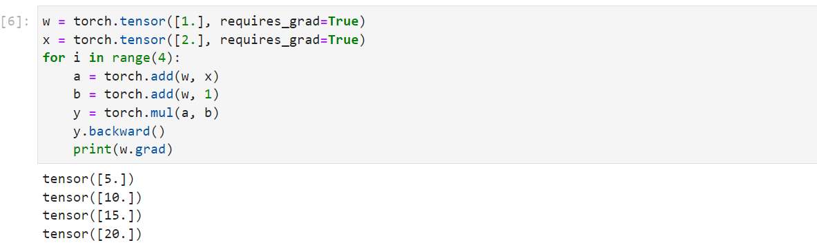
- 梯度不自动清零
1 | w = torch.tensor([1.], requires_grad=True) |
- 依赖于叶子结点的结点,requires_grad默认为True
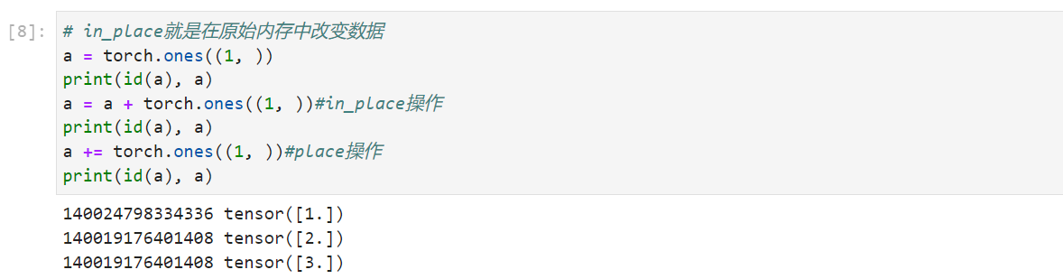
- 叶子结点不可执行in-place
1 | a = torch.ones((1, )) |
3.2逻辑回归
利用pytorch生成训练的数据
1 | import torch |
选择模型:
1 | #step2:模型 |
定义损失函数:
1 | #step3:损失函数 |
定义优化器:
1 | #step4:优化器 |
迭代训练模型
1 | #step5:迭代训练 |