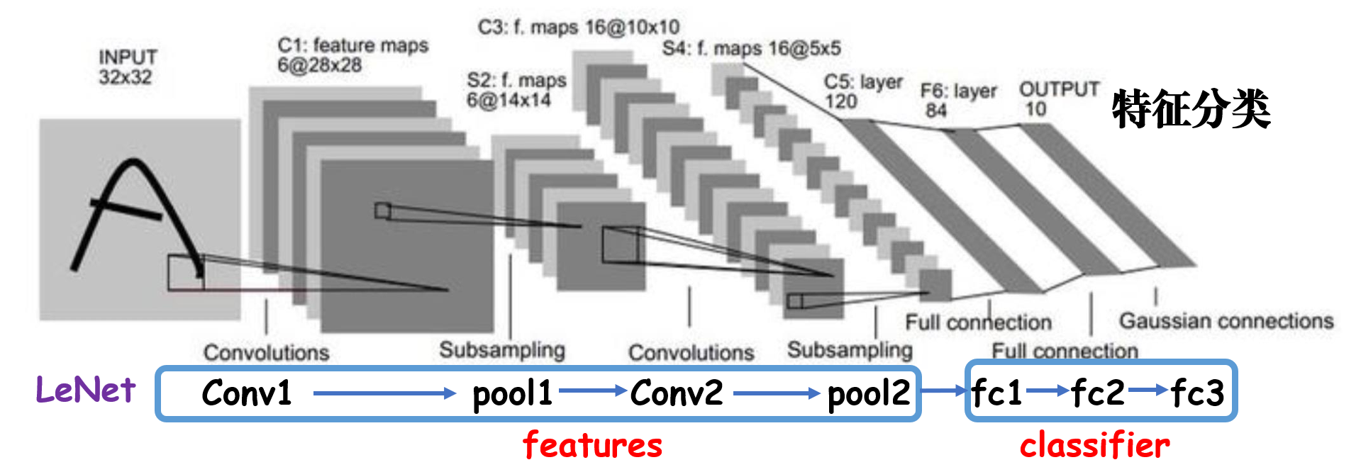
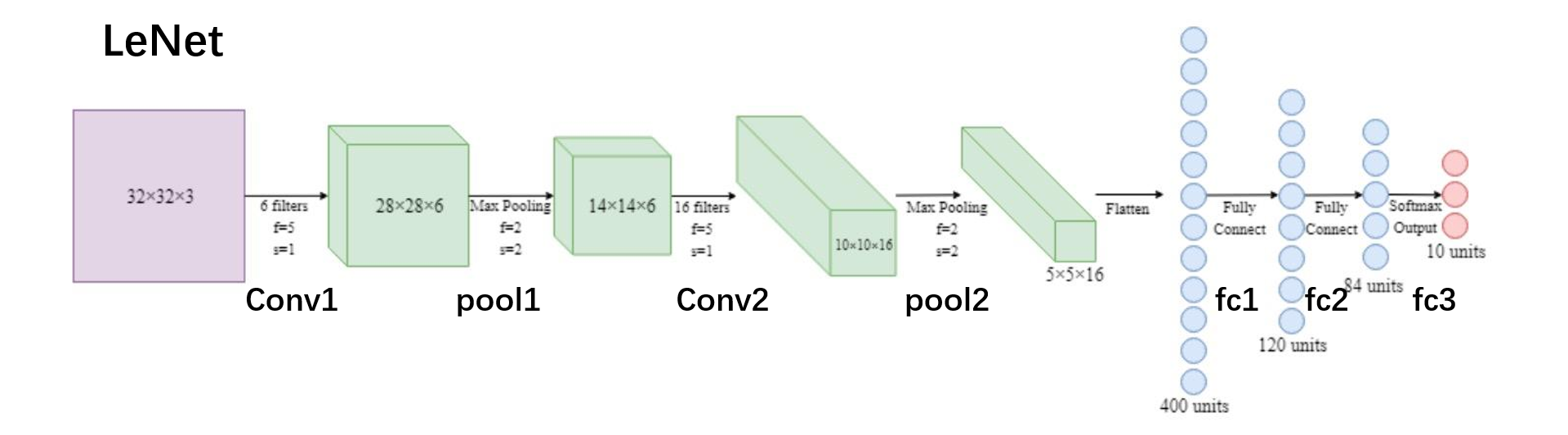
pytorch日积月累7-模型建立 1.1模型创建
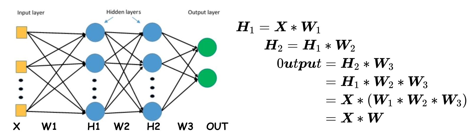
LeNet的计算图:(运算示意图)
1.2torch.nn torch.nn中包含以下四个主要部分:
nn.Module中的八个字典:
• parameters : 存储管理nn.Parameter类
• modules : 存储管理nn.Module类
• buffers:存储管理缓冲属性,如BN层中的running_mean
• ***_hooks:存储管理钩子函数
1
2
3
4
5
6
7
8
self._parameters = OrderedDict() self._buffers = OrderedDict() self._backward_hooks = OrderedDict() self._forward_hooks = OrderedDict() self._forward_pre_hooks = OrderedDict() self._state_dict_hooks = OrderedDict() self._load_state_dict_pre_hooks = OrderedDict() self._modules = OrderedDict()
nn.Module总结
一个module可以包含多个子module
一个module相当于一个运算,必须实现forward()函数
每个module都有8个字典管理它的属性
1.3模型容器Containers 模型容器Containers包含以下三个部分:
nn.Sequetial 按顺序包装多个网络层nn.ModuleDict 像python的dict一样包装多个网络层nn.ModuleList 像python的list一样包装多个网络层
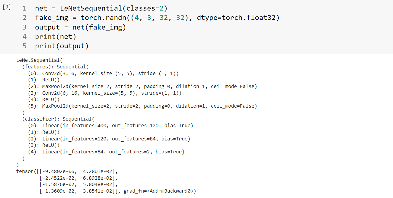
1.3.1 Sequential容器 Sequetial容器
1
2
3
4
5
6
7
8
9
10
11
12
13
14
15
16
17
18
19
20
21
22
23
24
25
26
class LeNetSequential (nn.Module): def __init__ (self, classes ): super (LeNetSequential, self).__init__() self.features = nn.Sequential( nn.Conv2d(3 , 6 , 5 ), nn.ReLU(), nn.MaxPool2d(kernel_size=2 , stride=2 ), nn.Conv2d(6 , 16 , 5 ), nn.ReLU(), nn.MaxPool2d(kernel_size=2 , stride=2 ), ) self.classifier = nn.Sequential( nn.Linear(16 *5 *5 , 120 ), nn.ReLU(), nn.Linear(120 , 84 ), nn.ReLU(), nn.Linear(84 , classes), ) def forward (self, x ): x = self.features(x) x = x.view(x.size()[0 ], -1 ) x = self.classifier(x) return x
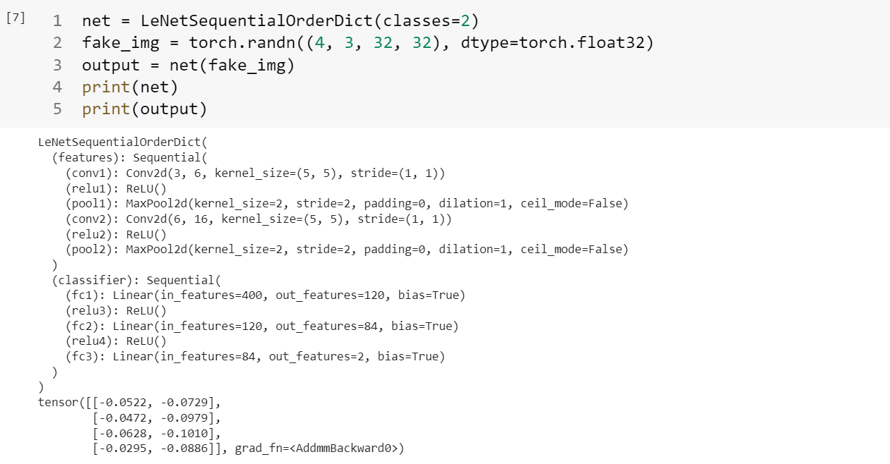
注意这种情况下每一层的输出都是按照序号来索引的,但是如果神经网络的层数很多的时候,这样的数字索引并不方便,所以采用下面的这种字典名称索引的方法:
1
2
3
4
5
6
7
8
9
10
11
12
13
14
15
16
17
18
19
20
21
22
23
24
from collections import OrderedDictclass LeNetSequentialOrderDict (nn.Module): def __init__ (self, classes ): super (LeNetSequentialOrderDict, self).__init__() self.features = nn.Sequential(OrderedDict({ 'conv1' : nn.Conv2d(3 , 6 , 5 ), 'relu1' : nn.ReLU(), 'pool1' : nn.MaxPool2d(kernel_size=2 , stride=2 ), 'conv2' : nn.Conv2d(6 , 16 , 5 ), 'relu2' : nn.ReLU(), 'pool2' : nn.MaxPool2d(kernel_size=2 , stride=2 ), })) self.classifier = nn.Sequential(OrderedDict({ 'fc1' : nn.Linear(16 *5 *5 , 120 ), 'relu3' : nn.ReLU(), 'fc2' : nn.Linear(120 , 84 ), 'relu4' : nn.ReLU(), 'fc3' : nn.Linear(84 , classes), })) def forward (self, x ): x = self.features(x) x = x.view(x.size()[0 ], -1 ) x = self.classifier(x) return x
nn.Sequential 是nn.module的容器,用于按顺序包装一组网络层
• 顺序性:各网络层之间严格按照顺序构建
• 自带forward():自带的forward里,通过for循环依次执行前向传播运算
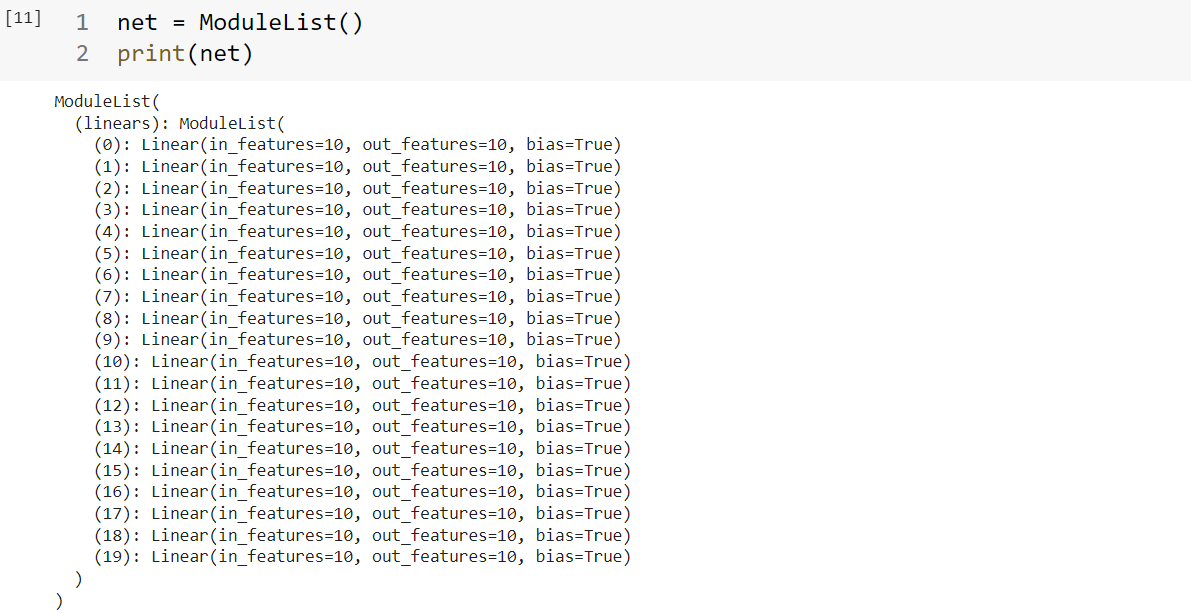
1.3.2 ModuleList容器 nn.ModuleList是nn.module的容器,用于包装一组网络层,以迭代方式调用网络层
主要方法:
• append():在ModuleList后面添加网络层
• extend():拼接两个ModuleList
• insert():指定在ModuleList中位置插入网络层
1
2
3
4
5
6
7
8
class ModuleList (nn.Module): def __init__ (self ): super (ModuleList, self).__init__() self.linears = nn.ModuleList([nn.Linear(10 , 10 ) for i in range (20 )]) def forward (self, x ): for i, linear in enumerate (self.linears): x = linear(x) return x
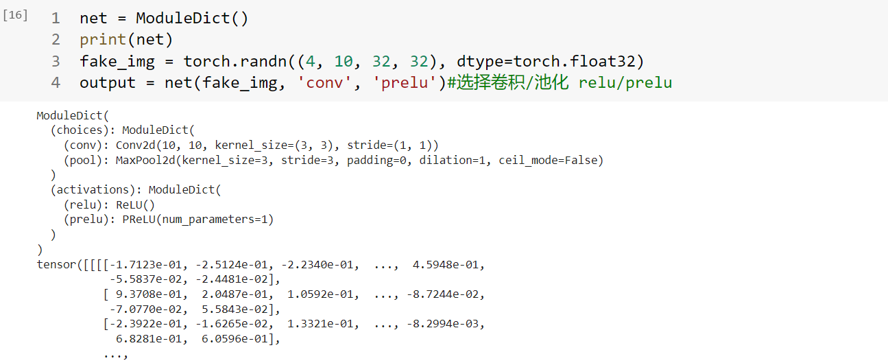
1.3.3 ModuleDict容器 是nn.module的容器,用于包装一组网络层,以索引方式调用网络层
主要方法:
• clear():清空ModuleDict
• items():返回可迭代的键值对(key-value pairs)
• keys():返回字典的键(key)
• values():返回字典的值(value)
• pop():返回一对键值,并从字典中删除
1
2
3
4
5
6
7
8
9
10
11
12
13
14
15
16
class ModuleDict (nn.Module): def __init__ (self ): super (ModuleDict, self).__init__() self.choices = nn.ModuleDict({ 'conv' : nn.Conv2d(10 , 10 , 3 ), 'pool' : nn.MaxPool2d(3 ) }) self.activations = nn.ModuleDict({ 'relu' : nn.ReLU(), 'prelu' : nn.PReLU() }) def forward (self, x, choice, act ): x = self.choices[choice](x) x = self.activations[act](x) return x
总结:
nn.Sequential:顺序性,各网络层之间严格按顺序执行,常用于block构建
nn.ModuleList:迭代性,常用于大量重复网构建,通过for循环实现重复构建
nn.ModuleDict:索引性,常用于可选择的网络层
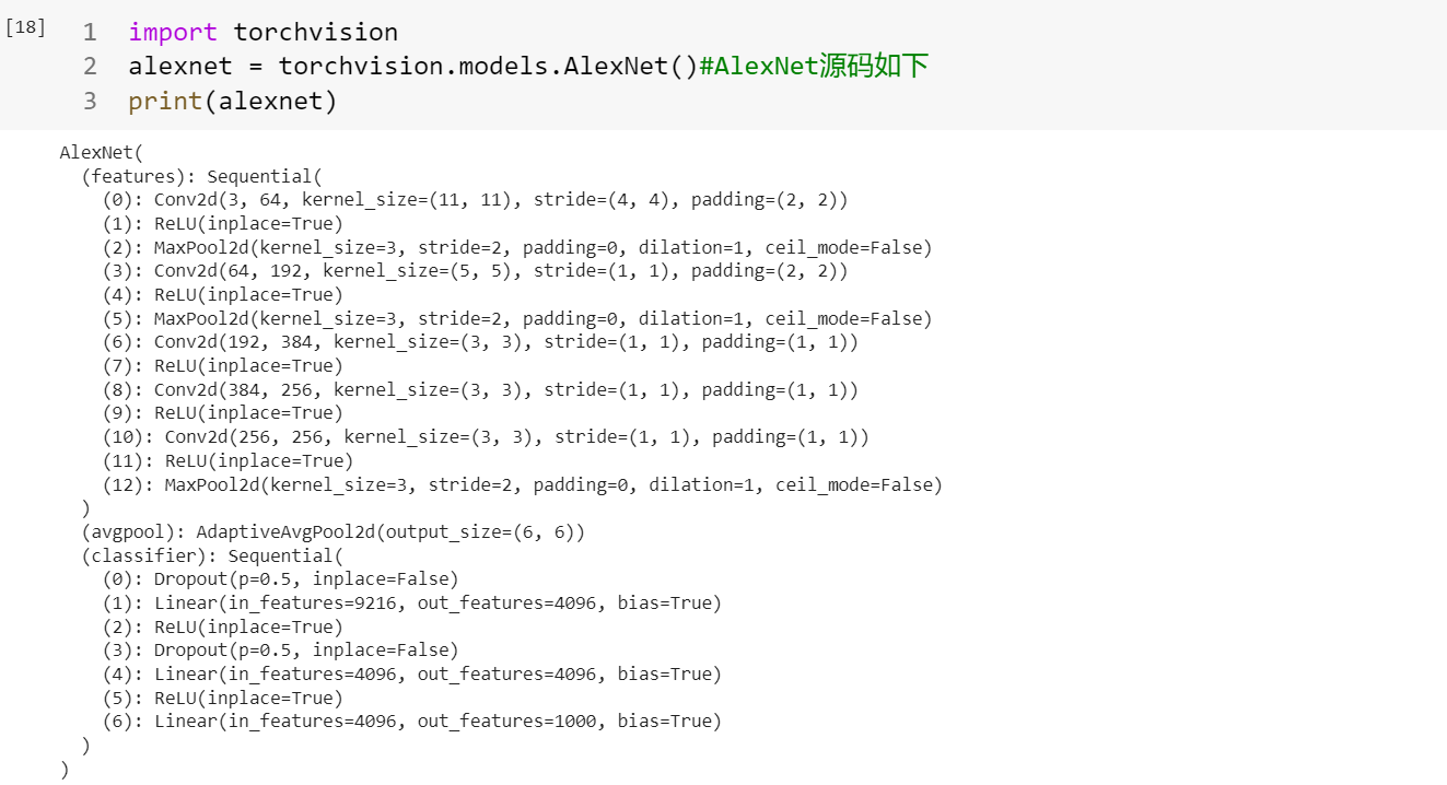
1.4AlexNet构建 1 2 import torchvisionalexnet = torchvision.models.AlexNet()
1 2 3 4 5 6 7 8 9 10 11 12 13 14 15 16 17 18 19 20 21 22 23 24 25 26 27 28 29 30 31 32 33 34 class AlexNet (nn.Module): def __init__ (self, num_classes=1000 ): super (AlexNet, self).__init__() self.features = nn.Sequential( nn.Conv2d(3 , 64 , kernel_size=11 , stride=4 , padding=2 ), nn.ReLU(inplace=True ), nn.MaxPool2d(kernel_size=3 , stride=2 ), nn.Conv2d(64 , 192 , kernel_size=5 , padding=2 ), nn.ReLU(inplace=True ), nn.MaxPool2d(kernel_size=3 , stride=2 ), nn.Conv2d(192 , 384 , kernel_size=3 , padding=1 ), nn.ReLU(inplace=True ), nn.Conv2d(384 , 256 , kernel_size=3 , padding=1 ), nn.ReLU(inplace=True ), nn.Conv2d(256 , 256 , kernel_size=3 , padding=1 ), nn.ReLU(inplace=True ), nn.MaxPool2d(kernel_size=3 , stride=2 ), ) self.avgpool = nn.AdaptiveAvgPool2d((6 , 6 )) self.classifier = nn.Sequential( nn.Dropout(), nn.Linear(256 * 6 * 6 , 4096 ), nn.ReLU(inplace=True ), nn.Dropout(), nn.Linear(4096 , 4096 ), nn.ReLU(inplace=True ), nn.Linear(4096 , num_classes), ) def forward (self, x ): x = self.features(x) x = self.avgpool(x) x = torch.flatten(x, 1 ) x = self.classifier(x) return x
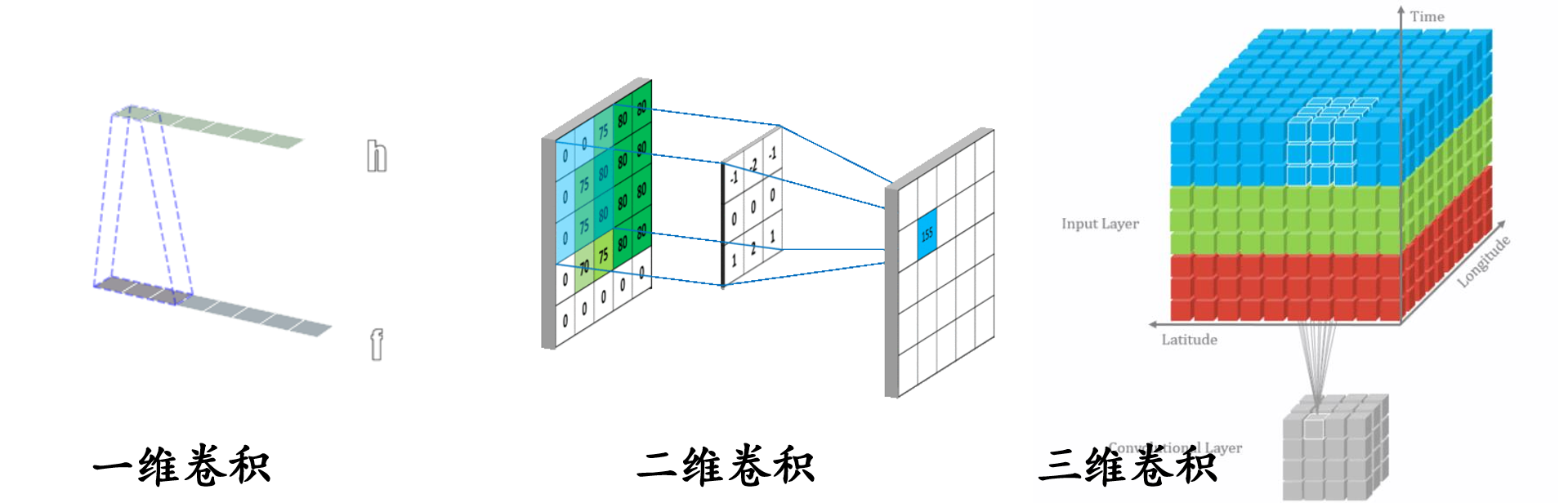
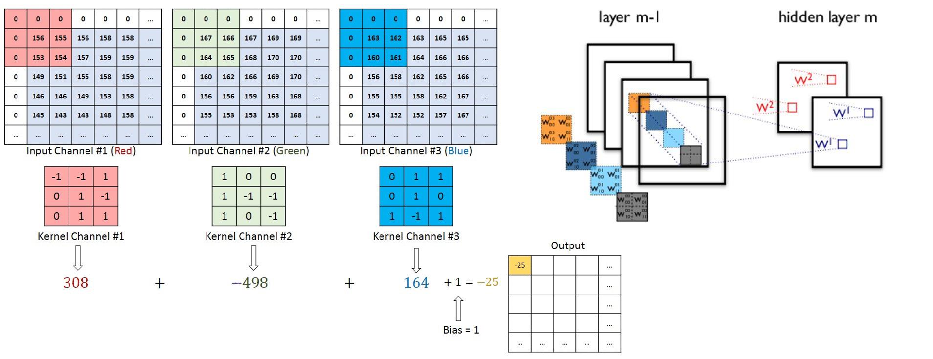
1.5卷积层 1.5.1 1d/2d/3d Convolution 卷积运算 :卷积核在输入信号(图像)上滑动,相应位置上进行乘加
卷积核 :又称为滤波器,过滤器,可认为是某种模式,某种特征。
卷积过程类似于用一个模版去图像上寻找与它相似的区域,与卷积核模式越相似,激活值越高,从而实现特征提取。
卷积维度:一般情况下,卷积核在几个维度上滑动, 就是几维卷积。
1.5.2 nn.Conv2d
1
2
3
4
5
6
7
8
9
nn.Conv2d(in_channels, out_channels, kernel_size, stride=1 , padding=0 , dilation=1 , groups=1 , bias=True , padding_mode='zeros' )
尺寸计算:
1
2
3
4
conv_layer = nn.Conv2d(3 , 1 , 3 ) nn.init.xavier_normal_(conv_layer.weight.data) img_conv = conv_layer(img_tensor)
卷积维度:一般情况下,卷积核在几个维度上滑动,就是几维卷积
转置卷积:
转置卷积又称为反卷积(Deconvolution)和部分跨越卷积(Fractionally strided Convolution) ,用于对图像进行上采样(UpSample)
为什么称为转置卷积?
假设图像尺寸为,卷积核为,padding=0,stride=1
正常卷积操作过程:图像:(先拉成向量)卷积核: 输出:
转置卷积: 假设图像尺寸为,卷积核为,padding=0,stride=1。图像:,卷积核: ,输出:
1
2
3
4
5
6
7
8
9
10
nn.ConvTranspose2d( in_channels, out_channels, kernel_size, stride=1 , padding=0 , output_padding=0 , groups=1 , bias=True , dilation=1 , padding_mode='zeros' )
尺寸计算简化版:
尺寸计算完整版:
1
2
3
4
conv_layer = nn.ConvTranspose2d(3 , 1 , 3 , stride=2 ) nn.init.xavier_normal_(conv_layer.weight.data) img_conv = conv_layer(img_tensor)
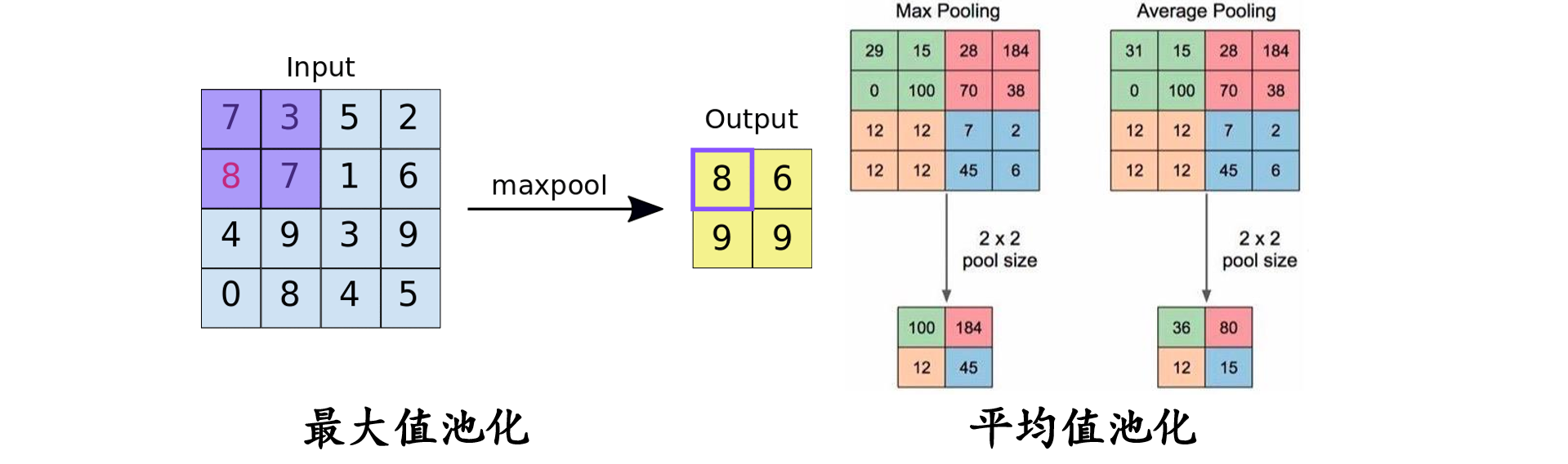
1.6池化层 池化运算:对信号进行收集”并“总结”,类似水池收集水资源,因而得名池化层
nn.MaxPool2d()功能:对二维图像信息进行最大值池化。
1 2 3 4 5 6 7 nn.MaxPool2d(kernel_size, stride=None , padding=0 , dilation=1 , return_indices=False , ceil_mode=False )
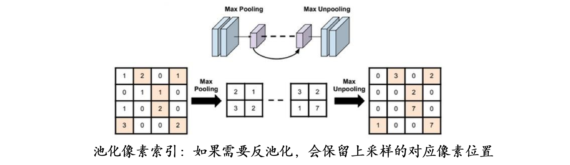
return_indices:记录池化像素索引,在反池化时,把对应的像素放在对应的位置上
1
2
3
maxpool_layer = nn.MaxPool2d((2 , 2 ), stride=(2 , 2 )) img_pool = maxpool_layer(img_tensor)
平均值池化:
1
2
3
4
5
6
nn.AvgPool2d(kernel_size, stride=None , padding=0 , ceil_mode=False , count_include_pad=True , divisor_override=None )
反池化:
1
2
3
4
nn.MaxUnpool2d( kernel_size, stride=None , padding=0 ) forward(self, input , indices, output_size=None )
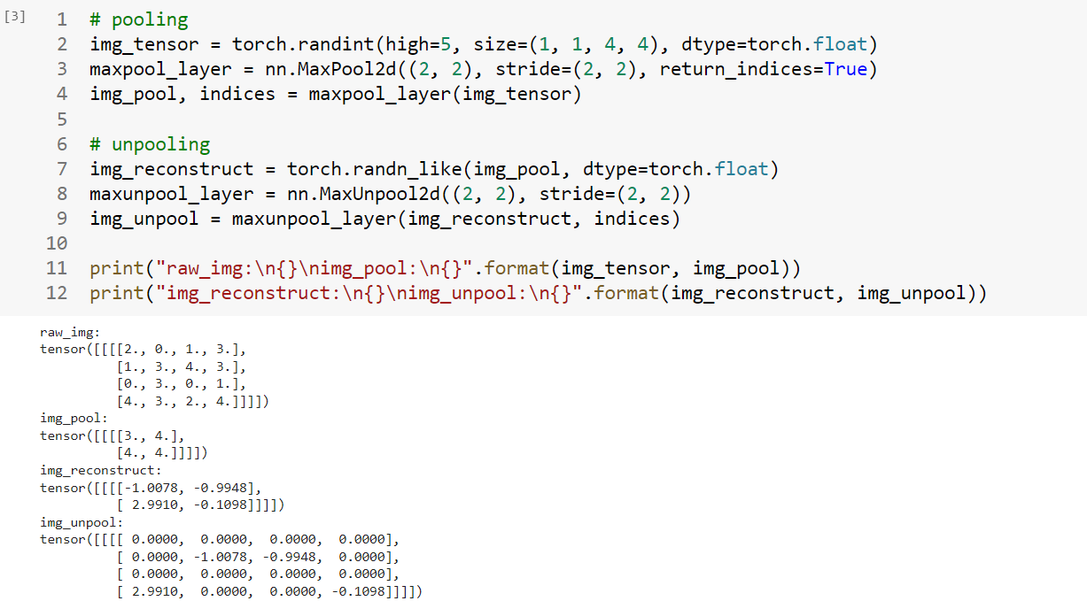
1 2 3 4 5 6 7 8 9 10 11 12 img_tensor = torch.randint(high=5 , size=(1 , 1 , 4 , 4 ), dtype=torch.float ) maxpool_layer = nn.MaxPool2d((2 , 2 ), stride=(2 , 2 ), return_indices=True ) img_pool, indices = maxpool_layer(img_tensor) img_reconstruct = torch.randn_like(img_pool, dtype=torch.float ) maxunpool_layer = nn.MaxUnpool2d((2 , 2 ), stride=(2 , 2 )) img_unpool = maxunpool_layer(img_reconstruct, indices) print ("raw_img:\n{}\nimg_pool:\n{}" .format (img_tensor, img_pool))print ("img_reconstruct:\n{}\nimg_unpool:\n{}" .format (img_reconstruct, img_unpool))
可以观察到img_unpool矩阵中对应的时矩阵中进行最大值池化的位置。
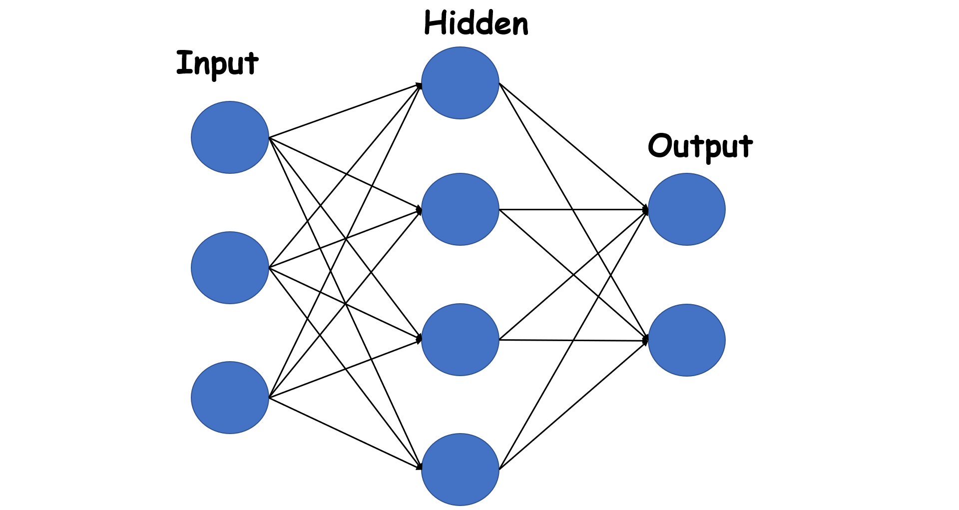
1.7线性层
线性层又称全连接层,其每个神经元与上一层所有神经元相连实现对前一层的线性组合,线性变换 。
1
2
3
nn.Linear(in_features, out_features, bias=True )
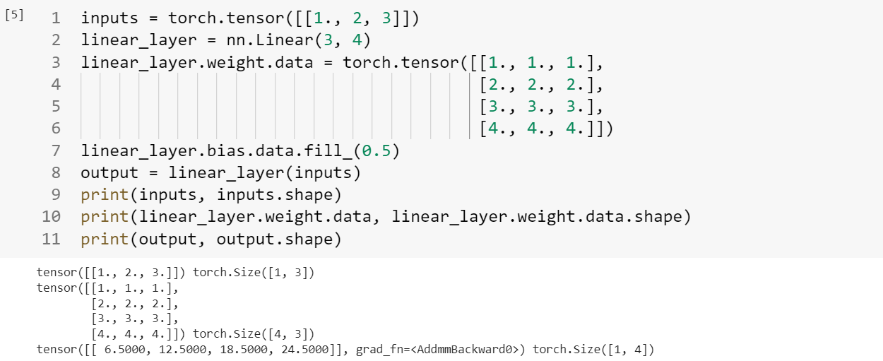
1
2
3
4
5
6
7
8
9
10
11
inputs = torch.tensor([[1. , 2 , 3 ]]) linear_layer = nn.Linear(3 , 4 ) linear_layer.weight.data = torch.tensor([[1. , 1. , 1. ], [2. , 2. , 2. ], [3. , 3. , 3. ], [4. , 4. , 4. ]]) linear_layer.bias.data.fill_(0.5 ) output = linear_layer(inputs) print (inputs, inputs.shape)print (linear_layer.weight.data, linear_layer.weight.data.shape)print (output, output.shape)
通过结果可以发现,线性层本质是$y=x W^{T}+\text{bias}$,如第一列为$1\times1+1\times2+1\times3=6$
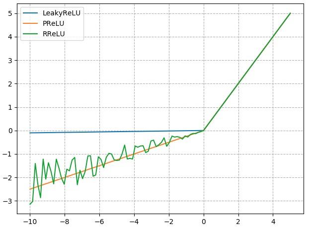
1.8激活函数层 激活函数对特征进行非线性变换,赋予多层神经网络具有深度的意义
常用的激活函数:
1
2
3
4
5
6
nn.Sigmoid() nn.tanh() nn.ReLu() nn.LeakyReLU() nn.PReLU() nn.RReLU()

 模型创建步骤: