CVbaseline-GoogleNet系列模型笔记

1.相关研究

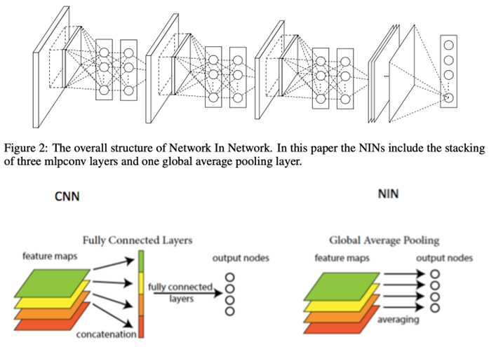
1.NIN(Network in Network)：首个采用$1\times 1$卷积的卷积神经网络，舍弃全连接层，大大减少网络参数。

特点：

$1\times 1$卷积
GAP输出（Global Average Pooling全局平均池化）

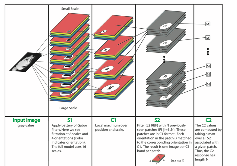
2.Robust Object Recognition with Cortex-Like Mechanisms ：多尺度Gabor滤波器提取特征

特点：S1层采用8种尺度Gabor滤波器进行提取不同尺度特征

3.Hebbian principle（赫布理论）：

“Cells that fire together, wire together”

(一起激发的神经元连接在一起)

2.研究成果

模型	时间	top-5
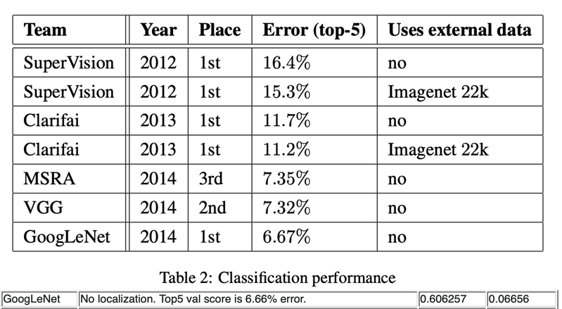
AlexNet	2012	15.3%
ZFNet	2013	13.5%
VGG	2014	7.3%
GoogLeNet	2014	6.6%

ILSVRC成绩：

GoogLeNet：分类第一名，检测第一名，定位第二名
VGG：定位第一名，分类第二名

研究意义：

开启多尺度卷积时代
拉开$1\times 1$卷积广泛应用序幕
为GoogLeNet系列开辟道路

3.摘要

本文主题：提出名为Inception的深度卷积神经网络，在ILSVRC-2014获得分类及检测双料冠军
模型特点1：Inception特点是提高计算资源利用率，增加网络深度和宽度时，参数少量增加
模型特点2：借鉴Hebbain理论和多尺度处理

4.GoogleNet结构

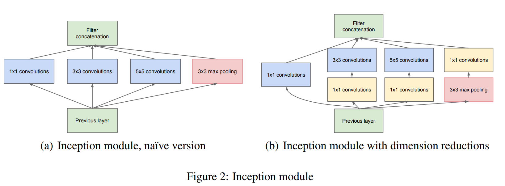
4.1 Inception module

特点：

多尺度（采用不同尺度的卷积核提取特征，多个分支进行处理）
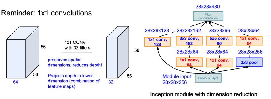
$1\times1$卷积降维，信息融合
$3\times3$max pooling保留了特征图数量

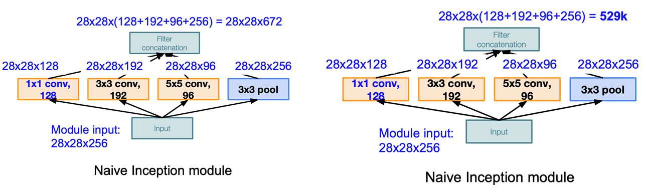
$3\times 3$ pool 可让特征图通道数增加，且用较少计算量

缺点：数据量（特征图）激增，计算量很大
解决方法：引入$1\times 1$卷积压缩厚度（试图减少卷积层输入的通道数量）。

Inception代码：

class Inception(nn.Module):
    __constants__ = ['branch2', 'branch3', 'branch4']

    def __init__(self, in_channels, ch1x1, ch3x3red, ch3x3, ch5x5red, ch5x5, pool_proj,
                 conv_block=None):
        super(Inception, self).__init__()
        if conv_block is None:
            conv_block = BasicConv2d
        # 定义四个分支
        # 1*1
        self.branch1 = conv_block(in_channels, ch1x1, kernel_size=1)    # 1*1

        # 3*3
        self.branch2 = nn.Sequential(
            conv_block(in_channels, ch3x3red, kernel_size=1),
            conv_block(ch3x3red, ch3x3, kernel_size=3, padding=1)
        )

        # 5*5 ；  kernel size 是 3*3
        self.branch3 = nn.Sequential(
            conv_block(in_channels, ch5x5red, kernel_size=1),
            conv_block(ch5x5red, ch5x5, kernel_size=3, padding=1)
        )

        # pool
        self.branch4 = nn.Sequential(
            nn.MaxPool2d(kernel_size=3, stride=1, padding=1, ceil_mode=True),
            conv_block(in_channels, pool_proj, kernel_size=1)
        )

    def _forward(self, x):
        branch1 = self.branch1(x)
        branch2 = self.branch2(x)
        branch3 = self.branch3(x)
        branch4 = self.branch4(x)

        outputs = [branch1, branch2, branch3, branch4]
        return outputs

    def forward(self, x):
        outputs = self._forward(x)
        # torch.cat(outputs, 1)在第一个维度，channel维度进行拼接
        return torch.cat(outputs, 1)

基本卷积层定义：

class BasicConv2d(nn.Module):
    def __init__(self, in_channels, out_channels, **kwargs):
        super(BasicConv2d, self).__init__()
        # nn.Conv2d的卷积
        self.conv = nn.Conv2d(in_channels, out_channels, bias=False, **kwargs)

    def forward(self, x):
        x = self.conv(x)
        return F.relu(x, inplace=True)

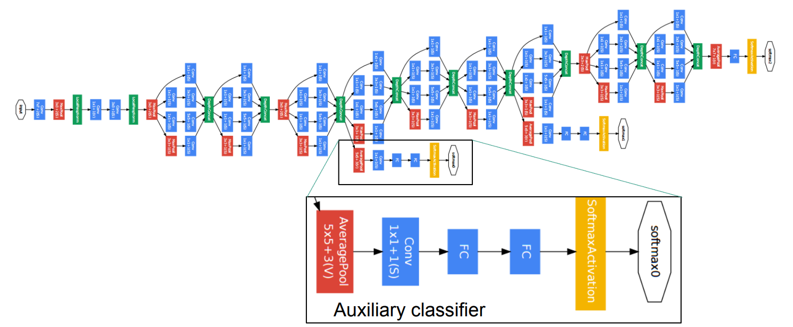
4.2 GoogLeNet

蓝色：卷积

红色：池化

绿色：LRN/特征融合

黄色：激活函数

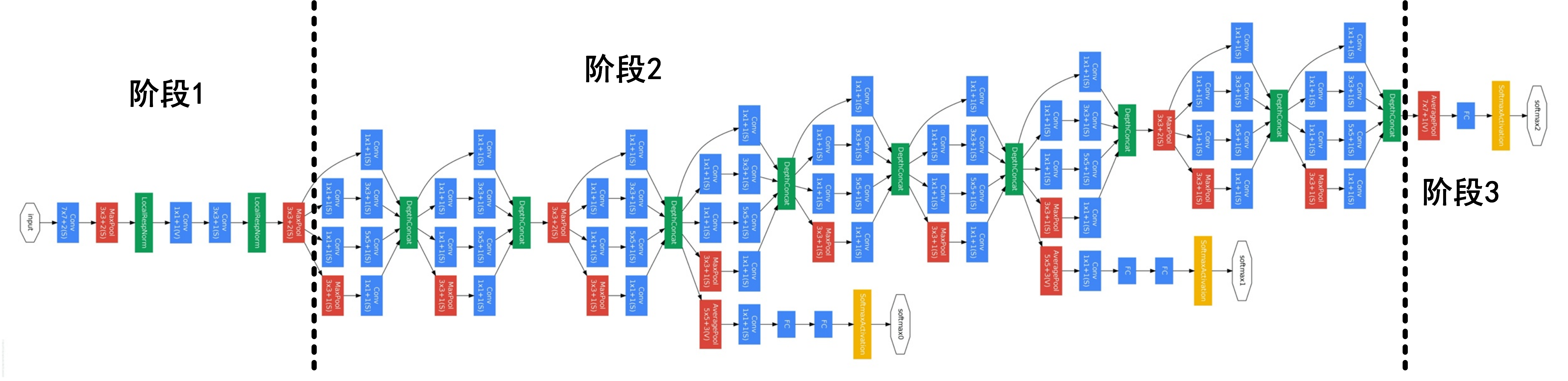
三阶段：

conv-pool-conv-pool 快速降低分辨率
堆叠Inception：堆叠使用Inception Module，达22层
FC层分类输出

附：增加两个辅助损失（图中下部的两个特殊分支），缓解梯度消失（中间层特征具有分类能力）

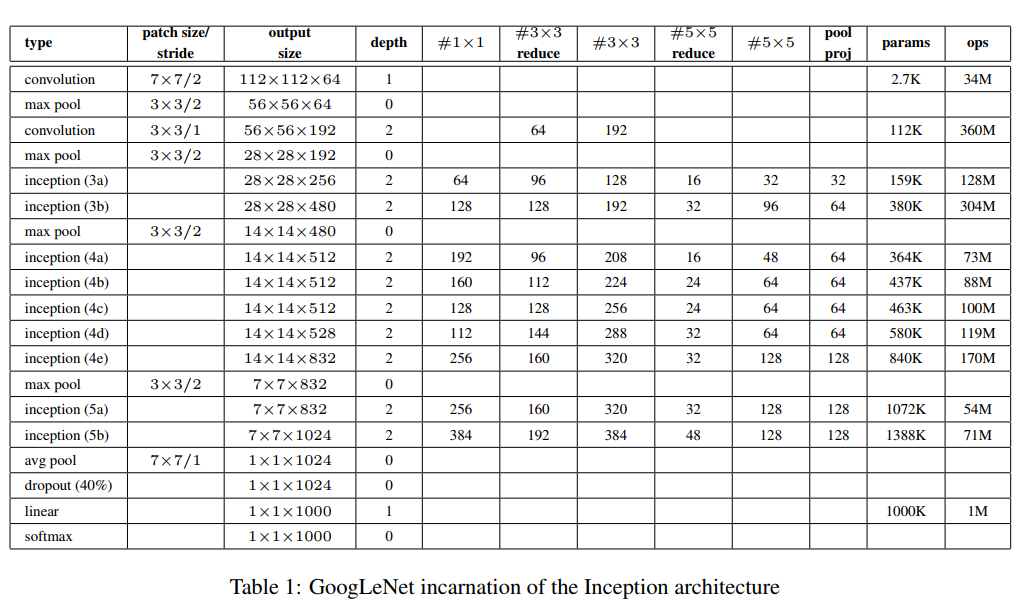
上面的结构特点：5个Block，5次分辨率下降，卷积核数量变化魔幻，输出层为1层FC层。

网络代码：

from collections import namedtuple
import torch
import torch.nn as nn
import torch.nn.functional as F
from torch.jit.annotations import Optional, Tuple
from torch import Tensor

GoogLeNetOutputs = namedtuple('GoogLeNetOutputs', ['logits', 'aux_logits2', 'aux_logits1'])
GoogLeNetOutputs.__annotations__ = {'logits': Tensor, 'aux_logits2': Optional[Tensor],
                                    'aux_logits1': Optional[Tensor]}
_GoogLeNetOutputs = GoogLeNetOutputs

# 类定义
class GoogLeNet(nn.Module):
    __constants__ = ['aux_logits', 'transform_input']

    def __init__(self, num_classes=1000, aux_logits=True, transform_input=False, init_weights=True,
                 blocks=None):
        super(GoogLeNet, self).__init__()
        if blocks is None:
            # 三个核心组件：卷积+Inception+Inception辅助损失
            blocks = [BasicConv2d, Inception, InceptionAux]   
            # 定义基本组件
        assert len(blocks) == 3
        
        conv_block = blocks[0]
        inception_block = blocks[1]
        inception_aux_block = blocks[2]

        self.aux_logits = aux_logits
        self.transform_input = transform_input
		# 第一阶段
        self.conv1 = conv_block(3, 64, kernel_size=7, stride=2, padding=3)
        self.maxpool1 = nn.MaxPool2d(3, stride=2, ceil_mode=True)
        self.conv2 = conv_block(64, 64, kernel_size=1)
        self.conv3 = conv_block(64, 192, kernel_size=3, padding=1)
        self.maxpool2 = nn.MaxPool2d(3, stride=2, ceil_mode=True)
        # 第二阶段
        self.inception3a = inception_block(192, 64, 96, 128, 16, 32, 32)
        self.inception3b = inception_block(256, 128, 128, 192, 32, 96, 64)
        self.maxpool3 = nn.MaxPool2d(3, stride=2, ceil_mode=True)
		# 第三阶段
        self.inception4a = inception_block(480, 192, 96, 208, 16, 48, 64)
        self.inception4b = inception_block(512, 160, 112, 224, 24, 64, 64)
        self.inception4c = inception_block(512, 128, 128, 256, 24, 64, 64)
        self.inception4d = inception_block(512, 112, 144, 288, 32, 64, 64)
        self.inception4e = inception_block(528, 256, 160, 320, 32, 128, 128)
        self.maxpool4 = nn.MaxPool2d(2, stride=2, ceil_mode=True)
		# 第四阶段
        self.inception5a = inception_block(832, 256, 160, 320, 32, 128, 128)
        self.inception5b = inception_block(832, 384, 192, 384, 48, 128, 128)

        if aux_logits:
            self.aux1 = inception_aux_block(512, num_classes)
            self.aux2 = inception_aux_block(528, num_classes)
		# 第五阶段
        self.avgpool = nn.AdaptiveAvgPool2d((1, 1))
        self.dropout = nn.Dropout(0.2)                     # 0.4 变为 0.2
        self.fc = nn.Linear(1024, num_classes)

        if init_weights:
            self._initialize_weights()

    def _initialize_weights(self):
        for m in self.modules():
            if isinstance(m, nn.Conv2d) or isinstance(m, nn.Linear):
                import scipy.stats as stats
                X = stats.truncnorm(-2, 2, scale=0.01)
                values = torch.as_tensor(X.rvs(m.weight.numel()), dtype=m.weight.dtype)
                values = values.view(m.weight.size())
                with torch.no_grad():
                    m.weight.copy_(values)
            elif isinstance(m, nn.BatchNorm2d):
                nn.init.constant_(m.weight, 1)
                nn.init.constant_(m.bias, 0)

    def _transform_input(self, x):
        # type: (Tensor) -> Tensor
        if self.transform_input:
            x_ch0 = torch.unsqueeze(x[:, 0], 1) * (0.229 / 0.5) + (0.485 - 0.5) / 0.5
            x_ch1 = torch.unsqueeze(x[:, 1], 1) * (0.224 / 0.5) + (0.456 - 0.5) / 0.5
            x_ch2 = torch.unsqueeze(x[:, 2], 1) * (0.225 / 0.5) + (0.406 - 0.5) / 0.5
            x = torch.cat((x_ch0, x_ch1, x_ch2), 1)
        return x

    def _forward(self, x):
        # type: (Tensor) -> Tuple[Tensor, Optional[Tensor], Optional[Tensor]]
        # N x 3 x 224 x 224
        x = self.conv1(x)
        # N x 64 x 112 x 112
        x = self.maxpool1(x)
        # N x 64 x 56 x 56
        x = self.conv2(x)
        # N x 64 x 56 x 56
        x = self.conv3(x)
        # N x 192 x 56 x 56
        x = self.maxpool2(x)

        # N x 192 x 28 x 28
        x = self.inception3a(x)
        # N x 256 x 28 x 28
        x = self.inception3b(x)
        # N x 480 x 28 x 28
        x = self.maxpool3(x)
        # N x 480 x 14 x 14
        x = self.inception4a(x)
        # N x 512 x 14 x 14
        # 只有在训练阶段才进行辅助损失
        aux_defined = self.training and self.aux_logits
        # 定义辅助损失
        if aux_defined:
            aux1 = self.aux1(x)
        else:
            aux1 = None

        x = self.inception4b(x)
        # N x 512 x 14 x 14
        x = self.inception4c(x)
        # N x 512 x 14 x 14
        x = self.inception4d(x)
        # N x 528 x 14 x 14
        # 是否进行辅助损失
        if aux_defined:
            aux2 = self.aux2(x)
        else:
            aux2 = None

        x = self.inception4e(x)
        # N x 832 x 14 x 14
        x = self.maxpool4(x)
        # N x 832 x 7 x 7
        x = self.inception5a(x)
        # N x 832 x 7 x 7
        x = self.inception5b(x)
        # N x 1024 x 7 x 7

        x = self.avgpool(x)
        # N x 1024 x 1 x 1
        x = torch.flatten(x, 1)
        # N x 1024
        x = self.dropout(x)
        x = self.fc(x)
        # N x 1000 (num_classes)
        return x, aux2, aux1

    @torch.jit.unused
    def eager_outputs(self, x, aux2, aux1):
        # type: (Tensor, Optional[Tensor], Optional[Tensor]) -> GoogLeNetOutputs
        if self.training and self.aux_logits:
            return _GoogLeNetOutputs(x, aux2, aux1)
        else:
            return x

    def forward(self, x):
        # type: (Tensor) -> GoogLeNetOutputs
        x = self._transform_input(x)        # 里面会判断是否需要transform
        x, aux1, aux2 = self._forward(x)    # 正式forwaord
        aux_defined = self.training and self.aux_logits
        if torch.jit.is_scripting():
            if not aux_defined:
                warnings.warn("Scripted GoogleNet always returns GoogleNetOutputs Tuple")
            return GoogLeNetOutputs(x, aux2, aux1)
        else:
            return self.eager_outputs(x, aux2, aux1)

5.训练技巧

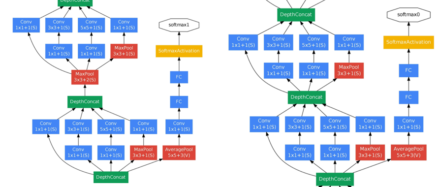
1.辅助损失：在Inception4b和Inception4e增加两个辅助分类层，用于计算辅助损失，达到：

增加loss回传
充当正则约束，迫使中间层特征也能具备分类能力

# 辅助损失定义 4a 4d
class InceptionAux(nn.Module):
    def __init__(self, in_channels, num_classes, conv_block=None):
        super(InceptionAux, self).__init__()
        if conv_block is None:
            conv_block = BasicConv2d
        self.conv = conv_block(in_channels, 128, kernel_size=1)
        self.fc1 = nn.Linear(2048, 1024)
        self.fc2 = nn.Linear(1024, num_classes)

    def forward(self, x):
        # aux1: N x 512 x 14 x 14, aux2: N x 528 x 14 x 14
        x = F.adaptive_avg_pool2d(x, (4, 4)) # 池化
        # aux1: N x 512 x 4 x 4, aux2: N x 528 x 4 x 4
        x = self.conv(x)
        # N x 128 x 4 x 4
        x = torch.flatten(x, 1)
        # N x 2048
        x = F.relu(self.fc1(x), inplace=True)
        # N x 1024
        x = F.dropout(x, 0.7, training=self.training)
        # N x 1024
        x = self.fc2(x)
        # N x 1000 (num_classes)
        return x

2.学习率下降策略：每8个epoch下降4%：fixed learning rate schedule (decreasing the learning rate by 4% every 8 epochs）$0.96^{100 }= 0.016$， 800个epochs，才下降不到100倍。

3.数据增强：指导方针如下：

图像尺寸均匀分布在8%-100%之间，进行随机裁剪。
长宽比在$[3/4, 4/3]$之间
光度畸变可以减轻过拟合，Photometric distortions 有效，如亮度、饱和度和对比度等

6.测试技巧

1. Multi crop：1张图变144张图

Step1: 等比例缩放短边至256, 288, 320, 352，四种尺寸。 一分为四

Step2: 在长边上裁剪出3个正方形，左中右或者上中下，三个位置。 一分为三

Step3: 左上，右上，左下，右下，中心，全局resize，六个位置。一分为六

Step4: 水平镜像。一分为二

$4\times 3\times 6\times 2 = 144$

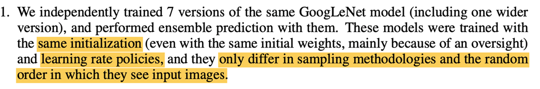
2. Model Fusion

七个模型训练差异仅在图像采样方式和顺序的差异

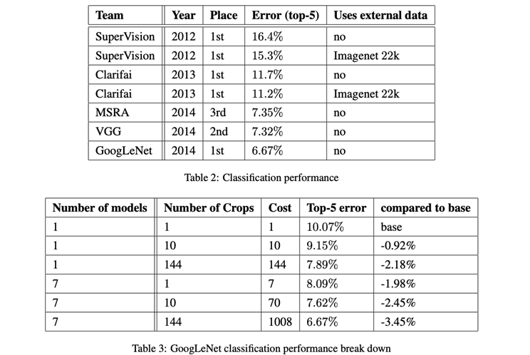
7.模型结果

分类结果：

模型融合：多模型比单模型精度高。
Multi Cros：crop越多，精度越高

检测结果：

模型融合：多模型比单模型精度高

8.稀疏结构

稀疏矩阵：数值为0的元素数目远远多于非0元素的数目，且无规律

稠密矩阵：数值非0的元素数目远远多于为0元素的数目，且无规律

稀疏矩阵优点是，可分解成密集矩阵计算来加快收敛速度。稀疏矩阵中0较多的区域就可以不用计算，计算量就大大降低。

特征图通道的分解

672个特征图分解为四个部分

$1\times1$卷积核提取的 128个通道
$3\times 3$ 卷积核提取的192个通道
$5\times 5$卷积核提取的96个通道
$3\times3$池化提取的256个通道

打破均匀分布，相关性强的特征聚集在一起

【思考】Inception的设计思路：

在直观感觉上在多个尺度上同时进行卷积，能提取到不同尺度的特征。特征更为丰富也意味着最后分类判断时更加准确。

利用稀疏矩阵分解成密集矩阵计算的原理来加快收敛速度。在inception上就是要在特征维度上进行分解。inception模块在多个尺度上提取特征，输出的256个特征就不再是均匀分布，而是相关性强的特征聚集在一起（比如$1\times1$的的96个特征聚集在一起，$3\times3$的96个特征聚集在一起，$5\times5$的64个特征聚集在一起）。这样的特征集中因为相关性较强的特征聚集在了一起，不相关的非关键特征就被弱化，同样是输出256个特征，inception方法输出的冗余信息较少。

Hebbin赫布原理。赫布认为“两个神经元或者神经元系统，如果总是同时兴奋，就会形成一种‘组合’，其中一个神经元的兴奋会促进另一个的兴奋”。在inception结构中就是要把相关性强的特征汇聚到一起，把$1\times1，3\times3，5\times5$的特征分开。因为训练收敛的最终目的就是要提取出独立的特征，所以预先把相关性强的特征汇聚，就能起到加速收敛的作用。

9.总结

关键点&创新点

大量使用$1\times1$，可降低维度，减少计算量，参数是AlexNet的是十二分之一
多尺度卷积核，实现多尺度特征提取
辅助损失层，增加梯度回传，增加正则，减轻过拟合

总结：

池化损失空间分辨率，但在定位、检测和人体姿态识别中仍应用。延伸拓展：定位、检测和人体姿态识别这些任务十分注重空间分辨率信息。

增加模型深度和宽度，可有效提升性能，但有2个缺点：容易过拟合，以及计算量过大

为节省内存消耗，先将分辨率降低，再堆叠使用Inception module

最后一个全连接层，是为了更方便的微调，迁移学习

网络中间层特征对于分类也具有判别性

学习率下降策略为每8个epochs下降4%（loss曲线很平滑）

数据增强指导方针：1. 尺寸在8%-100%；2. 长宽比在$[3/4, 4/3]$; 3. 光照畸变有效

随机采用差值方法可提升性能

实际应用中没必要144 crops

10.改进1 V2 批标准化

在GoogLeNet-V1 基础上加入BN层，同时借鉴VGG的小卷积核思想，将$5\times 5$卷积替换为2个$3\times3$卷积，提出了GoogLeNet-V2。

研究成果：

提出BN层：加快模型收敛，比googlenet-v1快数十倍，获得更优结果
GoogLeNet-v2 获得ILSVRC 分类任务 SOTA。BN使模型训练加快14倍，并且可显著提高分类精度，在Imagenet分类任务中超越了人类的表现。
开启神经网络设计新时代，标准化层已经成为深度神经网络标配。在Batch Normalization基础上拓展出了一系例标准化网络层，如Layer Normalization（LN），Instance Normalization（IN），Group Normalization（GN）

相关研究：

ICS（Internal Covariate Shift，内部协变量偏移）现象：输入数据分布变化，导致的模型训练困难，对深度神经网络影响极大。

白化（Whitening）：为了解决ICS，可以使用白化的方法，去除输入数据的冗余信息，使得数据特征之间的相关性较低，所有特征具有相同方差。依照概率论，$N(x)=(x-\text{mean}/\text{std})$，使得$x$变为0均值，1标准差。

BN 优点：

可以用更大学习率，加速模型收敛。针对类似Sigmoid的饱和激活函数，加上BN层后，可采用较大学习率。
可以不用精心设计权值初始化
可以不用dropout或较小的dropout。. 充当正则，顶替Dropout加入BN层后，将当前样本与以前样本通过统计信息联系起来，相当于某种约束，经实验表明可减轻Dropout的使用。
可以不用L2或者较小的weight decay
可以不用LRN(local response normalization)

10.1 BN层

批：一批数据，通常为mini-batch

标准化：使得分布为 mean=0， std=1

$\widehat{x}^{(k)}=\frac{x^{(k)}-\mathrm{E}\left[x^{(k)}\right]}{\sqrt{\operatorname{Var}\left[x^{(k)}\right]}}$

存在的问题：使神经元输出值在sigmod的线性区，削弱了网络的表达能力。
解决办法：$y^{(k)}=\gamma^{(k)}\widehat{x}^{(k)}+\beta^{(k)}$。采用可学习参数$\gamma$和$\beta$，增加线性变换，提升网络表达能力，同时提供恒等映射的可能（当$\gamma^{(k)}=\sqrt{\operatorname{Var}[x^{(k)}]}$和$\beta^{(k)}=\mathrm{E}[x^{(k)}]$时，BN层变为恒等映射，不改变神经元的输出值。$\widehat{x}^{(k)}=\frac{x^{(k)}-\mathrm{E}\left[x^{(k)}\right]}{\sqrt{\operatorname{Var}\left[x^{(k)}\right]}}$）

具体操作：

在mini-batch上计算均值
在mini-batch上计算标准差
减去均值，除以标准差，$\epsilon =1\times10^{-5}$，避免分母为0
线性变换，$\gamma$和$\beta$实现缩放与平移。

此时存在的问题：mini-batch的统计信息充当总体是不准确的

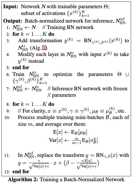
解决办法：采用指数滑动平均（Exponential Moving Average）来估计整体的均值，具体操作如下，公式中，$a_t$为当前值，$\text{mv}_t$为指数滑动平均值，$\text{decay}$控制权重衰减的速度。

$\begin{align} \text{mv}_t & = \text{decay}\times\text{mv}_{t-1}+(1-\text{decay})\times a_t\\ \text{mv}_t & = \sum_{i = 1}^t \text{decay}^{t-i}\times (1-\text{decay})\times a_t \end{align}$

展开表示为：

$\text{mv}_1=(1-\text{decay})a_1$
$\text{mv}_2=\text{decay}\times\text{mv}_1+ (1-\text{decay})a_2=\text{decay}(1-\text{decay})a_1+ (1-\text{decay})a_2$
$\text{mv}_3=\text{decay}^2(1-\text{decay})a_1+ \text{decay}(1-\text{decay})a_2+(1-\text{decay})a_3$
当$t-i>C$，$C$为无穷大的时候，有：
$\begin{align} & \text{decay}^{t-i} \times(1-\text{decay})\times a_t\approx 0\\ & \text{mv}_t \approx\sum_{i = t-C}^{t}\text{decay}^{t-i}\times(1-\text{decay})\times a_t \end{align}$

所以，算法的核心部分可以表示为：

$\begin{aligned} \widehat{x}_{i} & \leftarrow \frac{x_{i}-\mu_{\mathcal{B}}}{\sqrt{\sigma_{\mathcal{B}}^{2}+\epsilon}} \\ y_{i} & \leftarrow \widehat{x}_{i}+\beta \equiv \mathrm{BN}_{\gamma, \beta}\left(x_{i}\right) \end{aligned}$

算法的整体流程如下：

10.2 GoogleNetV2网络结构

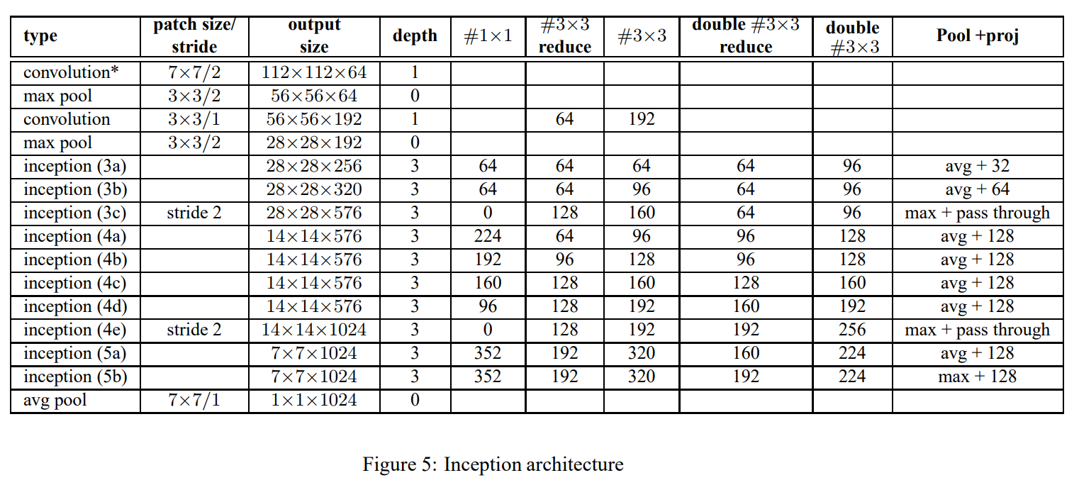
对V1的改进：

激活函数前加入BN

$5\times5$卷积替换为2个$3\times3$卷积（小卷积核结构）

第一个Inception模块增加一个Inception结构

增多$5\times5$卷积核

尺寸变化采用stride=2的卷积（不再使用池化操作）

增加9层（10-1层）到 31层（10表示inception数量），使用了更多的卷积核

加入BN的卷积层：

class BasicConv2d(nn.Module):

    def __init__(self, in_channels, out_channels, **kwargs):
        super(BasicConv2d, self).__init__()
        self.conv = nn.Conv2d(in_channels, out_channels, bias=False, **kwargs)
        self.bn = nn.BatchNorm2d(out_channels, eps=0.001)  # googlenet-v2

    def forward(self, x):
        x = self.conv(x)
        x = self.bn(x)  # googlenet-v2
        return F.relu(x, inplace=True)

10.3 实验

其使用的是tanh激活函数，从下图中可以发现：

红色为未加入BN层的，在几个epoch后，其分布主要集中在两侧，说明已经落入了激活函数的饱和区间（在后面的几个epoch中，如>6个epoch后，梯度很小，梯度不会更新了），而加入BN层后，可以拉至0均值附近，避免进入饱和区，其分布会相对均匀。

bn_tanh

10.4 nn.batchnorm

torch.nn.BatchNorm1d(num_features, 
                     eps=1e-05, 
                     momentum=0.1, 
                     affine=True, 
                     track_running_stats=True)

num_features – 一个样本的特征数量（最重要！！）
eps – 为数值稳定性而加到分母上的值$\epsilon$。
momentum – 移动平均的动量值。
affine – 一个布尔值，当设置为真时，此模块具有可学习的仿射参数。

torch.nn.BatchNorm2d(num_features, eps=1e-05, momentum=0.1, 
                     affine=True, 
                     track_running_stats=True, 
                     device=None, dtype=None)

torch.nn.BatchNorm3d(num_features, eps=1e-05, momentum=0.1, 
                     affine=True, 
                     track_running_stats=True, 
                     device=None, dtype=None)

说明：此处的更新方式与论文中略有不同：

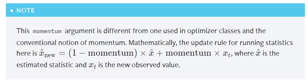
11.改进2 V3 改进Inception

研究成果：

1.提出Inception-V2 和 Inception-V3， Inception-V3模型获得 ILSVRC 分类任务SOTA

2.提出4个网络模型设计准则，为模型设计提供参考

3.提出卷积分解、高效降低特征图分辨率方法和标签平滑技巧，提升网络速度与精度

模型	时间	top-5
AlexNet	2012	15.3%
ZFNet	2013	13.5%
VGG	2014	7.3%
GoogLeNet	2014	6.6%
GoogLeNet v2	2015	4.9%
GoogLeNet v3	2015	3.5%

总结：网络设计准则：

1.尽量避免信息瓶颈，通常发生在池化层，即特征图变小，信息量减少，类似一个瓶颈。

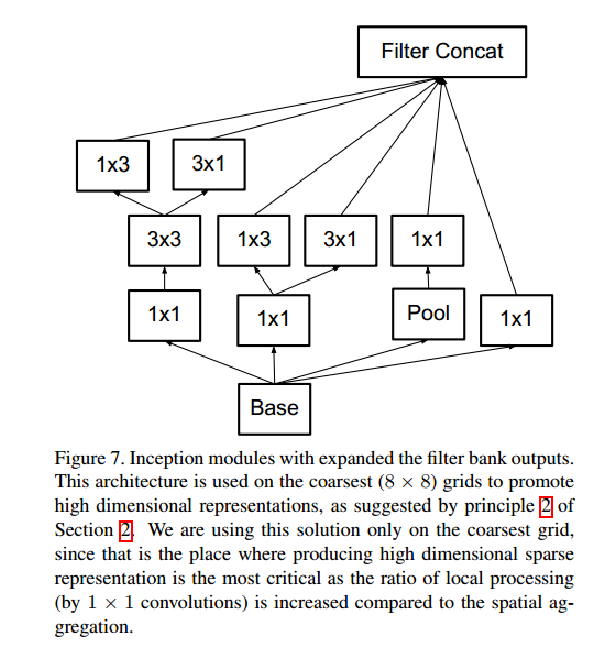
2.采用更高维的表示方法能够更容易的处理网络的局部信息。

3.大的卷积核可以分解为数个小卷积核，且不会降低网络能力。

4.把握好深度和宽度的平衡。

11.1 卷积分解

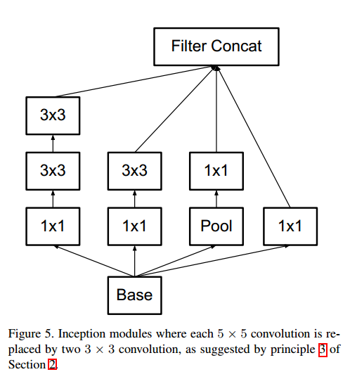
第一种分解：大卷积核分解为小卷积核堆叠，1个$5\times5$卷积分解为2个$3\times3$卷积，参数减少$1 -(9+9)/25 = 0.28%$（在VGG中有详细的介绍）
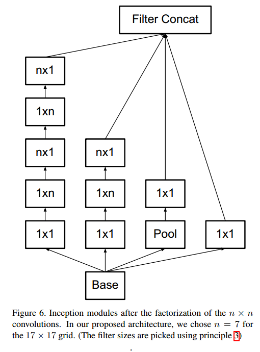
第二种分解：分解为非对称卷积（Asymmetric Convolutionals）1个$n\times n$卷积分解为$1\times n$卷积和$n\times 1$卷积堆叠。对于$3\times 3$而言，参数减少 $1 - (3+3)/9 = 0.33$。注意事项：非对称卷积在后半段使用效果才好，特别是特征图分辨率在$12\sim20$之间，本文在分辨率为$17\times17$的时候使用非对称卷积分解。

11.2 辅助分类层的改进

GoogleNetV1中提出辅助分类层，用于缓解梯度消失，提升底层的特征提取能力，本文对辅助分类层进行分析，得出结论：

辅助分类层在初期起不到作用，在后期才能提升网络性能，因此移除第一个辅助分类层不影响精度。
辅助分类层可辅助低层提取特征是不正确的
辅助分类层对模型起到正则的作用
googlenet-v3只在$17\times17$特征图结束接入辅助分类层

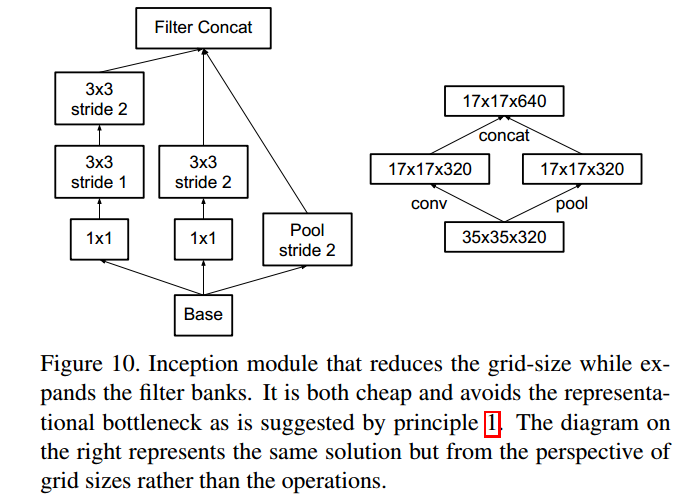
11.3 高效特征图下降策略

特征图下降方式探讨：传统池化方法存在信息表征瓶颈（representational bottlenecks）问题（违反模型设计准则1），即特征图信息变少了。
- 简单解决方法：先用卷积将特征图通道数翻倍，再用池化。
- 存在问题：计算量过大
- 解决方法：用卷积得到一半的特征图，用池化得到另一半的特征图。

高效特征图分辨率下降策略：用卷积得到一半特征图，用池化得到一半特征图。用较少的计算量获得较多的信息，避免信息表征瓶颈（ representational bottlenecks）
- 该Inception-module用于$35\times 35$下降至$17\times 17$，以及$17\times17$下降至$8\times8$。下图中右侧为左侧的简化：

11.4 标签平滑

传统的ont-hot编码中存在的问题：导致过拟合

提出了标签平滑，把one-hot中概率为1的那一项进行衰减，衰减的那部分自信度平均分到每一个类别中。

举例：4分类任务，$\text{label}=(0,1,0,0)$

标签平滑后：

$\begin{align} \text{label Smoothing} & = (0.001/4,1-0.001+0.001/4,0.001/4,0.001/4)\\ & = (0.00025,0.99925,0.00025,0.00025) \end{align}$

标签平滑公式：

交叉熵（Cross Entropy）：$H(q,p)=-\sum_{k=1}^k\log(p_k)q_k$，其中$q$为one-hot向量。

标签平滑：将$q$标签平滑为$q’$，让模型输出的$p$分布去逼近$q’$

$q’(k|x)=(1-\varepsilon )\delta_{k,y}+\varepsilon u(k)$，其中$u(k)$为一个概率分布，这里如果采用均匀分布，则可以得到：$q’(k|x)=(1-\varepsilon )\delta_{k,y}+\frac{\varepsilon }{k}$
所以标签平滑后的交叉熵损失函数为：

推导：

即：

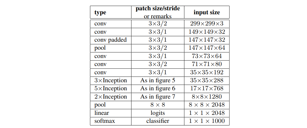
$H(q',p)=-\sum_{k=1}^k\log(p_k)q'_k=(1-\varepsilon )H(q,p)+\varepsilon H(q',p)$

11.5 模型结构

针对V1的变化：

采用3个$3\times3$卷积替换1个$7\times 7$卷积，并且在第一个卷积就采用stride=2来降低分辨率
第二个$3\times3$卷积，在第2个卷积才下降分辨率
第一个block增加一个inception-module，第一个inception-module只是将$5\times5$卷积替换为2个$3\times3$卷积。
第二个block，处理$17\times17$特征图，采用非对称卷积。
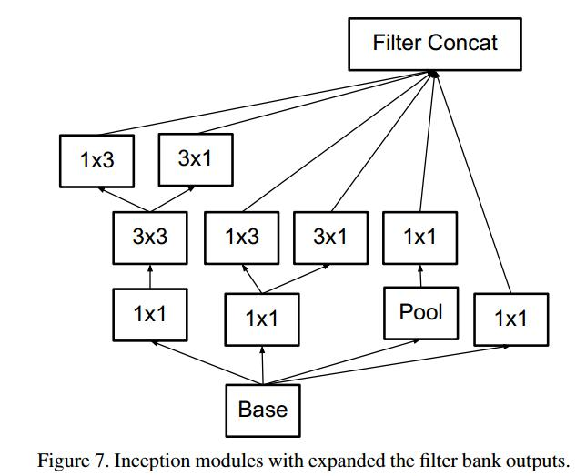
第三个block，处理$8\times8$特征图，遵循准则2，提出拓展的卷积
最后输出2048个神经元（V1是1024个神经元）

拓展的卷积结构如下（InceptionV2结构）：

Inception V3对V2的改进：

采用RMSProp优化方法
采用Label Smoothing正则化方法
采用非对称卷积提取$17\times17$特征图
采用带BN的辅助分类层

11.6 各个Inception结构的代码

核心部分代码：只保留了init和forward两个函数

class Inception3(nn.Module):
    def __init__(self, num_classes=1000, aux_logits=True, transform_input=False, init_weights=False,
                 inception_blocks=None):
        super(Inception3, self).__init__()
        if inception_blocks is None:
            # inception核心组件！！！
            inception_blocks = [
                BasicConv2d, InceptionA, InceptionB, InceptionC,
                InceptionD, InceptionE, InceptionAux
            ]
        assert len(inception_blocks) == 7
        conv_block = inception_blocks[0]
        inception_a = inception_blocks[1]
        inception_b = inception_blocks[2]
        inception_c = inception_blocks[3]
        inception_d = inception_blocks[4]
        inception_e = inception_blocks[5]
        inception_aux = inception_blocks[6]

        self.aux_logits = aux_logits
        self.transform_input = transform_input
        
        self.Conv2d_1a_3x3 = conv_block(3, 32, kernel_size=3, stride=2)
        self.Conv2d_2a_3x3 = conv_block(32, 32, kernel_size=3)
        self.Conv2d_2b_3x3 = conv_block(32, 64, kernel_size=3, padding=1)
        self.Conv2d_3b_1x1 = conv_block(64, 80, kernel_size=1)
        self.Conv2d_4a_3x3 = conv_block(80, 192, kernel_size=3)

        self.Mixed_5b = inception_a(192, pool_features=32)
        self.Mixed_5c = inception_a(256, pool_features=64)
        self.Mixed_5d = inception_a(288, pool_features=64)

        self.Mixed_6a = inception_b(288)
        self.Mixed_6b = inception_c(768, channels_7x7=128)
        self.Mixed_6c = inception_c(768, channels_7x7=160)
        self.Mixed_6d = inception_c(768, channels_7x7=160)
        self.Mixed_6e = inception_c(768, channels_7x7=192)

        if aux_logits:
            self.AuxLogits = inception_aux(768, num_classes)

        self.Mixed_7a = inception_d(768)
        self.Mixed_7b = inception_e(1280)
        self.Mixed_7c = inception_e(2048)
        
        self.fc = nn.Linear(2048, num_classes)

        if init_weights:
            self._initialize_weights()

    def _forward(self, x):

        # 1/5
        # N x 3 x 299 x 299
        x = self.Conv2d_1a_3x3(x)
        # N x 32 x 149 x 149
        x = self.Conv2d_2a_3x3(x)
        # N x 32 x 147 x 147
        x = self.Conv2d_2b_3x3(x)
        # N x 64 x 147 x 147
        x = F.max_pool2d(x, kernel_size=3, stride=2)
        # N x 64 x 73 x 73
        x = self.Conv2d_3b_1x1(x)
        # N x 80 x 73 x 73
        x = self.Conv2d_4a_3x3(x)
        # N x 192 x 71 x 71
        x = F.max_pool2d(x, kernel_size=3, stride=2)

        # 2/5
        # N x 192 x 35 x 35
        x = self.Mixed_5b(x)
        # N x 256 x 35 x 35
        x = self.Mixed_5c(x)
        # N x 288 x 35 x 35
        x = self.Mixed_5d(x)

        # 3/5
        # N x 288 x 35 x 35
        x = self.Mixed_6a(x)
        # N x 768 x 17 x 17
        x = self.Mixed_6b(x)
        # N x 768 x 17 x 17
        x = self.Mixed_6c(x)
        # N x 768 x 17 x 17
        x = self.Mixed_6d(x)
        # N x 768 x 17 x 17
        x = self.Mixed_6e(x)


        # N x 768 x 17 x 17
        aux_defined = self.training and self.aux_logits
        if aux_defined:
            aux = self.AuxLogits(x)
        else:
            aux = None

        # 4/5
        # N x 768 x 17 x 17
        x = self.Mixed_7a(x)
        # N x 1280 x 8 x 8
        x = self.Mixed_7b(x)
        # N x 2048 x 8 x 8
        x = self.Mixed_7c(x)


        # 5/5
        # N x 2048 x 8 x 8
        # Adaptive average pooling
        x = F.adaptive_avg_pool2d(x, (1, 1))
        # N x 2048 x 1 x 1
        x = F.dropout(x, training=self.training)
        # N x 2048 x 1 x 1
        x = torch.flatten(x, 1)
        # N x 2048
        x = self.fc(x)
        # N x 1000 (num_classes)
        return x, aux

（核心）基本组件：InceptionA、InceptionB、InceptionC、InceptionD、InceptionE、InceptionAux、BasicConv2d

InceptionA

代码与论文的差异:

(1) $3\times3$卷积部分多了1个$3\times3$卷积；

(2) $5\times5$卷积并没有用2个$3\times3$卷积替换

class InceptionA(nn.Module):

    def __init__(self, in_channels, pool_features, conv_block=None):
        super(InceptionA, self).__init__()
        if conv_block is None:
            conv_block = BasicConv2d
        self.branch1x1 = conv_block(in_channels, 64, kernel_size=1)

        self.branch5x5_1 = conv_block(in_channels, 48, kernel_size=1)
        # 5*5卷积并没有用2个3*3卷积替换
        self.branch5x5_2 = conv_block(48, 64, kernel_size=5, padding=2)

        #3*3卷积部分多了1个3*3卷积
        self.branch3x3dbl_1 = conv_block(in_channels, 64, kernel_size=1)
        self.branch3x3dbl_2 = conv_block(64, 96, kernel_size=3, padding=1)
        self.branch3x3dbl_3 = conv_block(96, 96, kernel_size=3, padding=1)

        self.branch_pool = conv_block(in_channels, pool_features, kernel_size=1)

    def _forward(self, x):
        branch1x1 = self.branch1x1(x)

        branch5x5 = self.branch5x5_1(x)
        branch5x5 = self.branch5x5_2(branch5x5)

        branch3x3dbl = self.branch3x3dbl_1(x)
        branch3x3dbl = self.branch3x3dbl_2(branch3x3dbl)
        branch3x3dbl = self.branch3x3dbl_3(branch3x3dbl)

        branch_pool = F.avg_pool2d(x, kernel_size=3, stride=1, padding=1)
        branch_pool = self.branch_pool(branch_pool)

        outputs = [branch1x1, branch5x5, branch3x3dbl, branch_pool]
        return outputs

    def forward(self, x):
        outputs = self._forward(x)
        return torch.cat(outputs, 1)

inceptionB

inceptionC

inceptionE

附：论文原文

GoogleNetV1：

GoogleNetV2：加入BN层

GoogleNetV3：改进Inception，提出InceptionV2，InceptionV3