Text Classification
1. 概述
- Text Classification is a technique of categorizing natural language texts into pre-defined, organized groups
- In other words - it is the activity of labeling texts with categories from a pre-defined set, based upon the content
Classic examples include classification of books in libraries or segmentation of articles in news,by looking at the content.
Text classification is a sub-field of text analytics, which uses machine learning to extract meaning from text documents
- Text classification technique has been used successfully for:
- Sentiment analysis
- Topic detection
- Language detection
- Fraud, Profanity, and Emergency detection
- Urgency detection in customer support
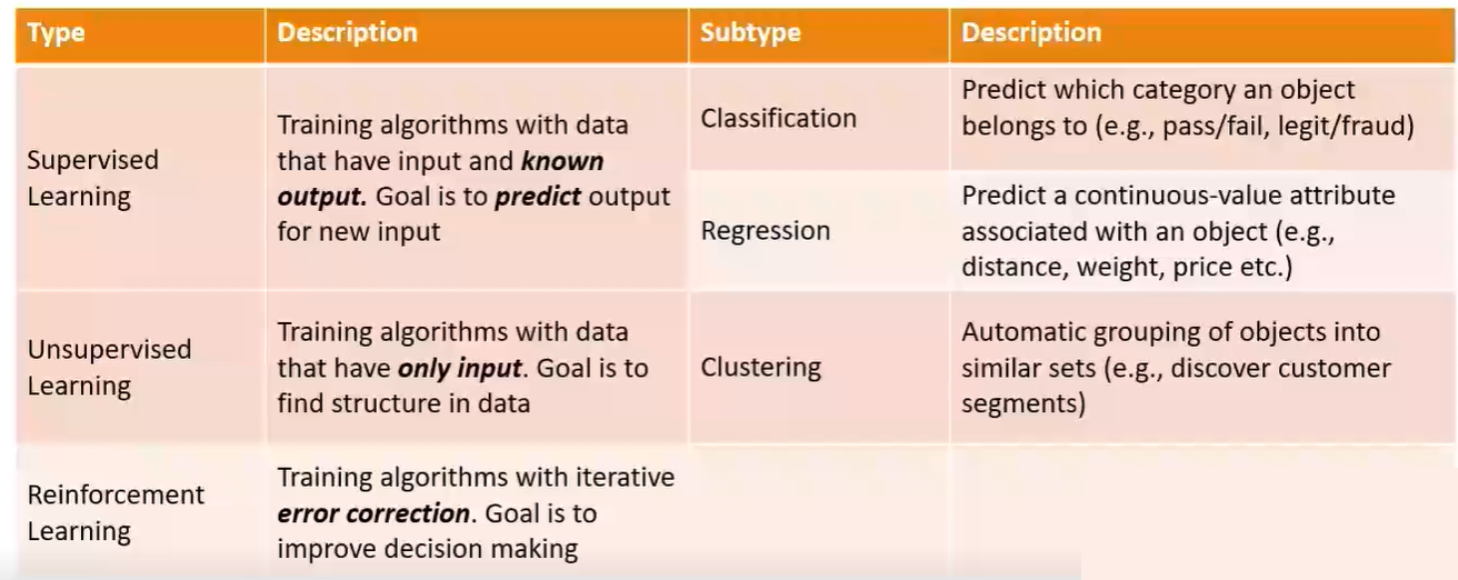
2. Machine Learning
参考链接:
machine learning for NLP
- Processing natural language text is complex, and the traditional rules-based, explicit programming is not practical
- Machine Learning allows algorithms to iteratively learn from text and extract rules, instead of explicitly programming for it
- Machine learning can improve, accelerate and automate NLP tasks and text analytics functions
Core NLP tasks are performed with machine learning models:

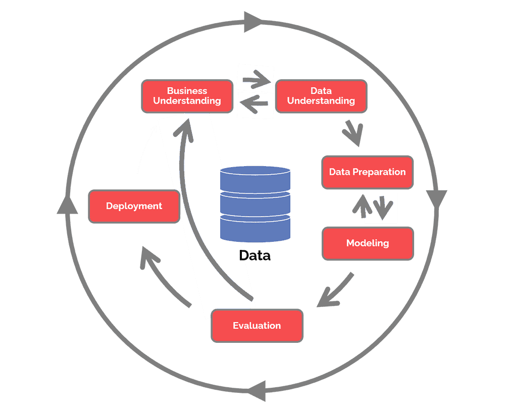
Machine Learning Process:CRISP-DM
- The Cross-Industry-StandardProcess-for-Data-Mining (CRISP-DM), a well-established scientific method
- Process Steps are:
- Business Understanding
- Data Understanding
- Data Preparation
- Modeling
- Evaluation
- Deployment
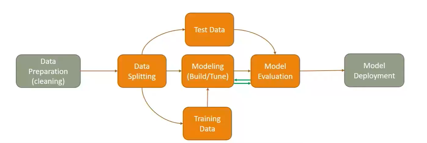
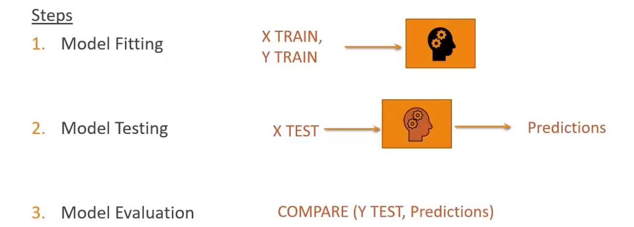
Model Building & Evaluation Deep Dive
3. Classification Modeling Example
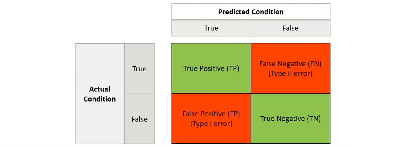
model evaluation-Confusion Matrix
For the classification problem,you predict either right or wrong-however,there are two dimensions to evaluate the result.
#Correct Predictions/Total # Predictions Ability to find all relevant cases within
dataset. Tells us how complete the result is Ability to find only the relevant data points. Tells us how valid the result is
Harmonic mean of recall and precision
| Metric | Definition | Calculations using confusion matrix |
|---|---|---|
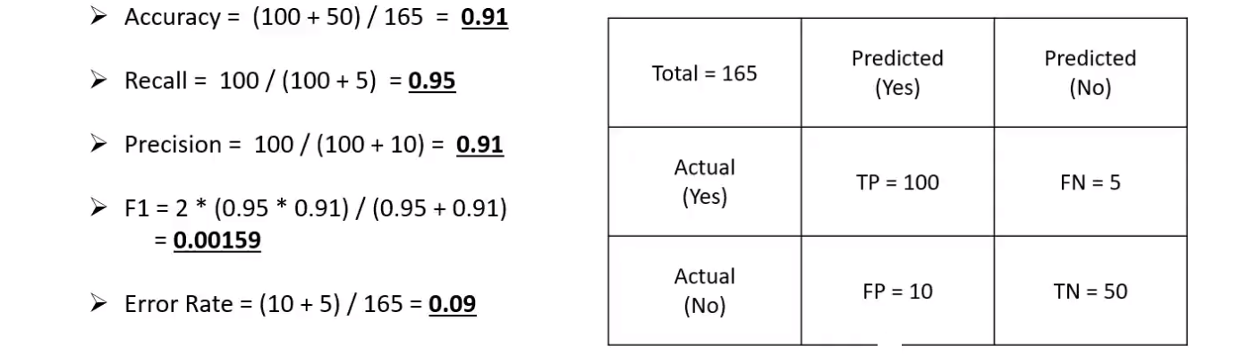
| Accuracy | #Correct Predictions/Total # Predictions | $(TP+TN)/Total$ |
| Recall(sensitivity) | Ability to find all relevant cases within dataset. Tells us how complete the result is | $(TP)/(TP+FN)$ |
| Precision | Ability to find only the relevant data points. Tells us how valid the result is | $(TP)/(TP+FP)$ |
| F1-Score | Harmonic mean of recall and precision | $F1=2\times \frac{\text{precision}\times\text{recall}}{\text{precision}+\text{recall}}$ |
An example:
4. scikit-learn
安装:
1 | pip install scikit-learn |
Scikit usage steps(5 high level steps)
select a model(estimator object)
1
2
from sklearn.linear_model import LinearRegression
model = LinearRegression(normalize = True)Split the data into test and training sets
1
2
from sklearn.model_selection import train_test_split
X_train, X_test, y_train, y_test = train_test_split(X, y, test_size = 0.3)Train/fit the model
1
model.fit(X_train, t_train)
Predict Labels for test data
1
predictions = model.predict(X_test)
Evaluate model(create metrics)
sklearn demo
1 | import numpy as np |
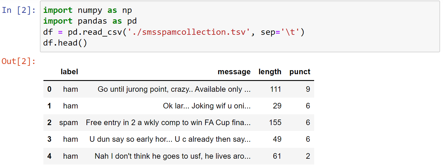
1 | # 查看是否有缺失的数据 |
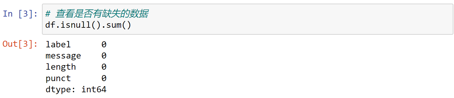
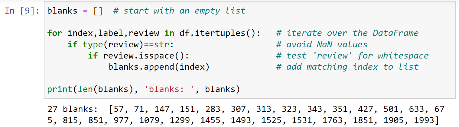
可以看到此时数据集中没有空缺项,如果有空缺项,可以使用下面的代码补充空缺:
1 | blanks = [] # start with an empty list |
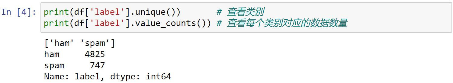
1 | print(df['label'].unique()) # 查看类别 |
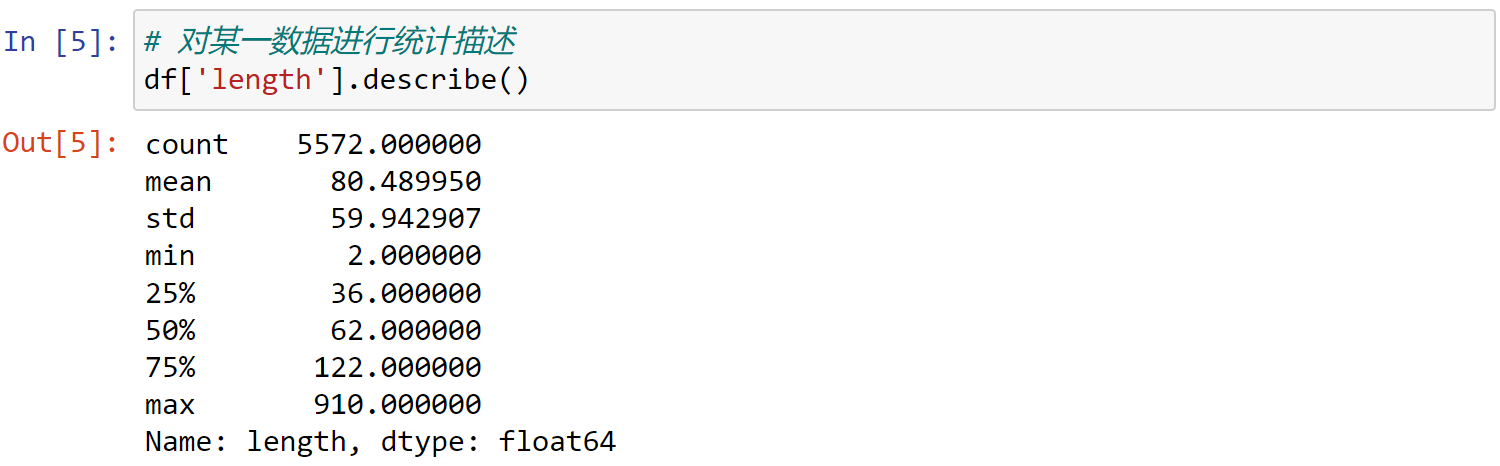
1 | # 对某一数据进行统计描述 |
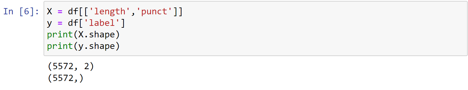
1 | X = df[['length','punct']] |
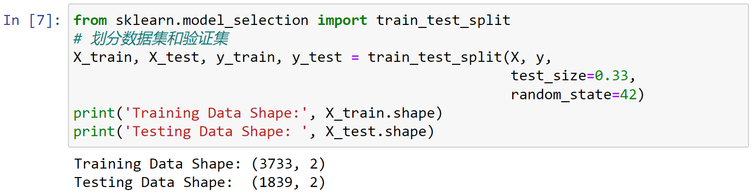
1 | from sklearn.model_selection import train_test_split |
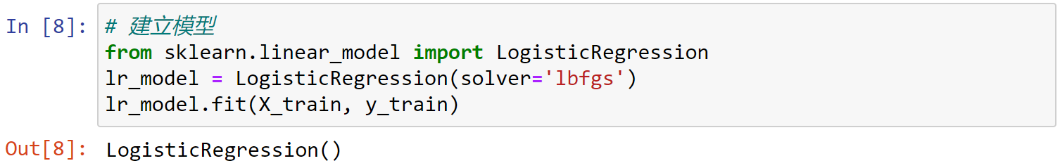
创建一个LogisticRegression模型
1 | # 建立模型 |
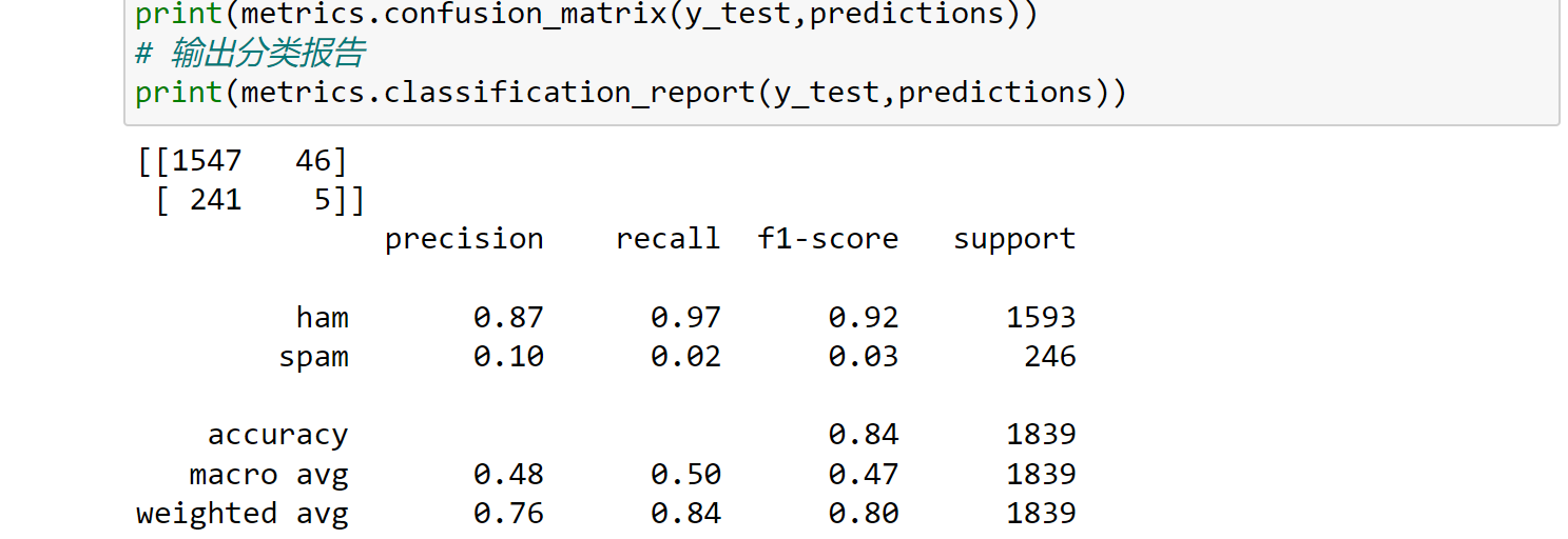
1 | from sklearn import metrics |
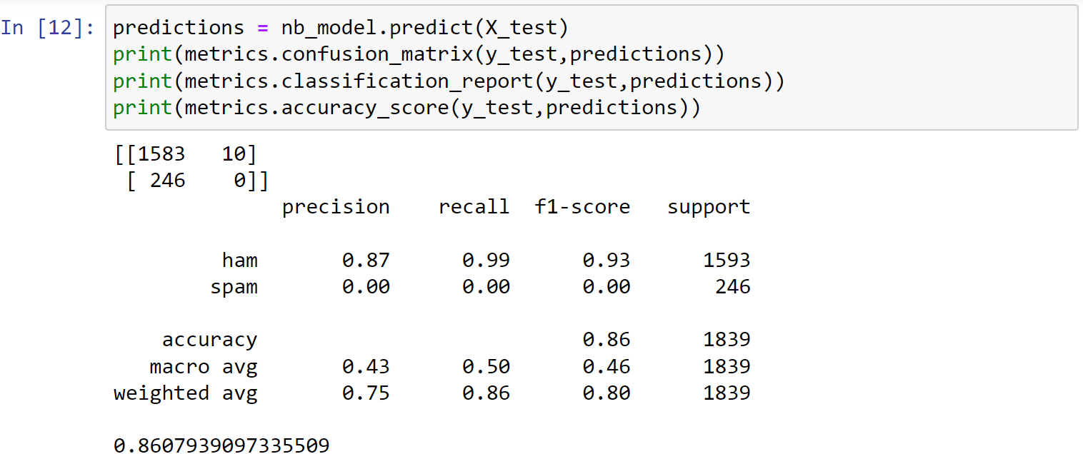
创建一个朴素贝叶斯模型naïve Bayes classifier
1 | # Train a naïve Bayes classifier: |
1 | predictions = nb_model.predict(X_test) |
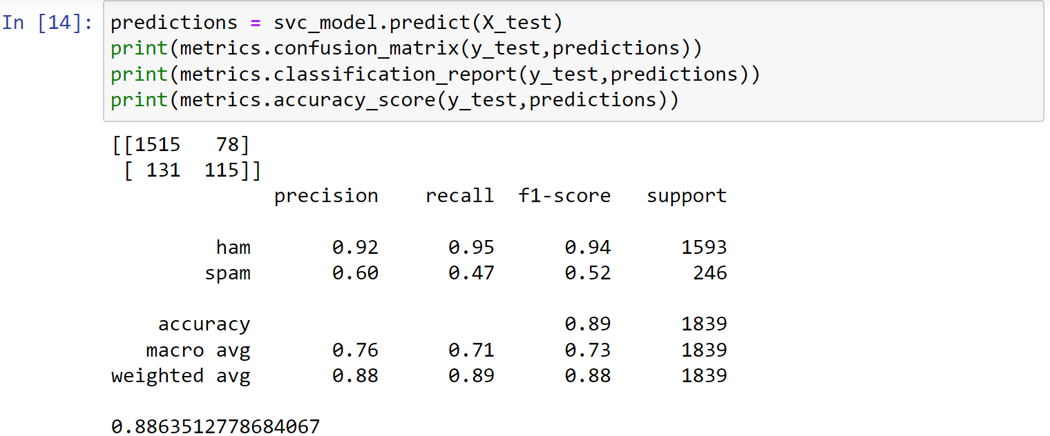
创建一个支持向量机模型svc
1 | from sklearn.svm import SVC |
1 | predictions = svc_model.predict(X_test) |
5. Text Feature Extraction
- Machine learning algorithms (models) need numerical features to perform learning and prediction activities
- We need to extract numerical features from the raw text
5.1 count vectorization
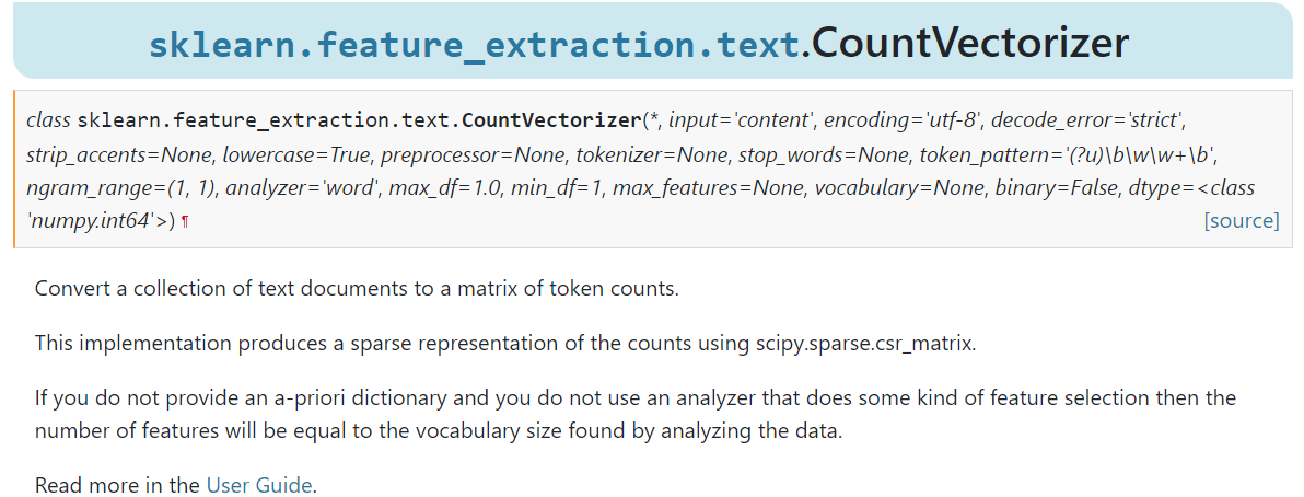
CountVectorizer 类:
- create a matrix of counts,with columns as words,会将文本中的词语转换为词频矩阵
- 矩阵中包含一个元素
a[i][j],它表示j词在i类文本下的词频。This sparse matrix is called Document Term Matrix(DTM) fit_transform函数计算各个词语出现的次数get_feature_names()可获取词袋中所有文本的关键字,toarray()可看到词频矩阵的结果。
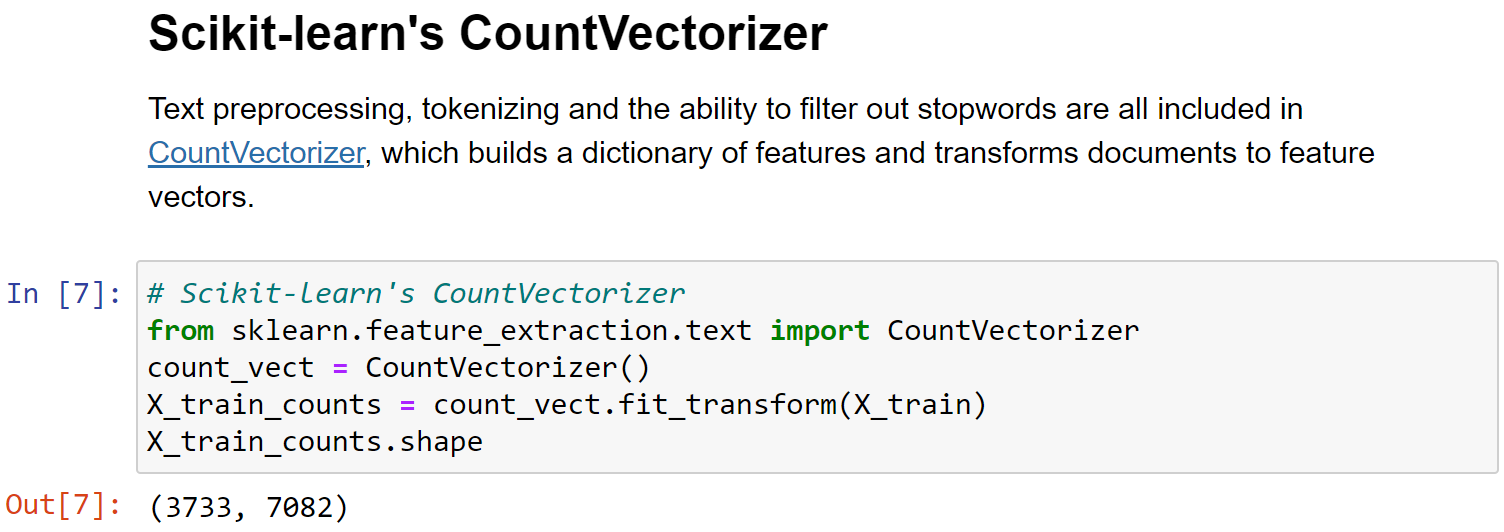
1 | # Scikit-learn's CountVectorizer |
5.2 Term Frequency(TF)
- Term Frequency
tf(t,d)-raw count of a term in a document, i.e.,the number of times a termtoccurs in documentd - However,Term Frequency alone is not enough for a thorough feature analysis of the text. Consider stop words like “a” or “the”
- Because the term “the” is so common, term frequency will tend to incorrectly emphasize documents which happen to use the word “the” more frequently, without giving enough weight to the more meaningful terms “red” and “dogs”.
5.3 Inverse Document Frequency(IDF)
- In order to reduce the unwanted impact of common words, an inverse document frequency factor is incorporated which diminishes the weight of terms that occur very frequently in the document set and increases the weight of terms that occur rarely
- It is the logarithmically scaled inverse fraction of the documents that contain the word (obtained by dividing the total number of documents by the number of documents containing the term, and then taking the logarithm of that quotient)
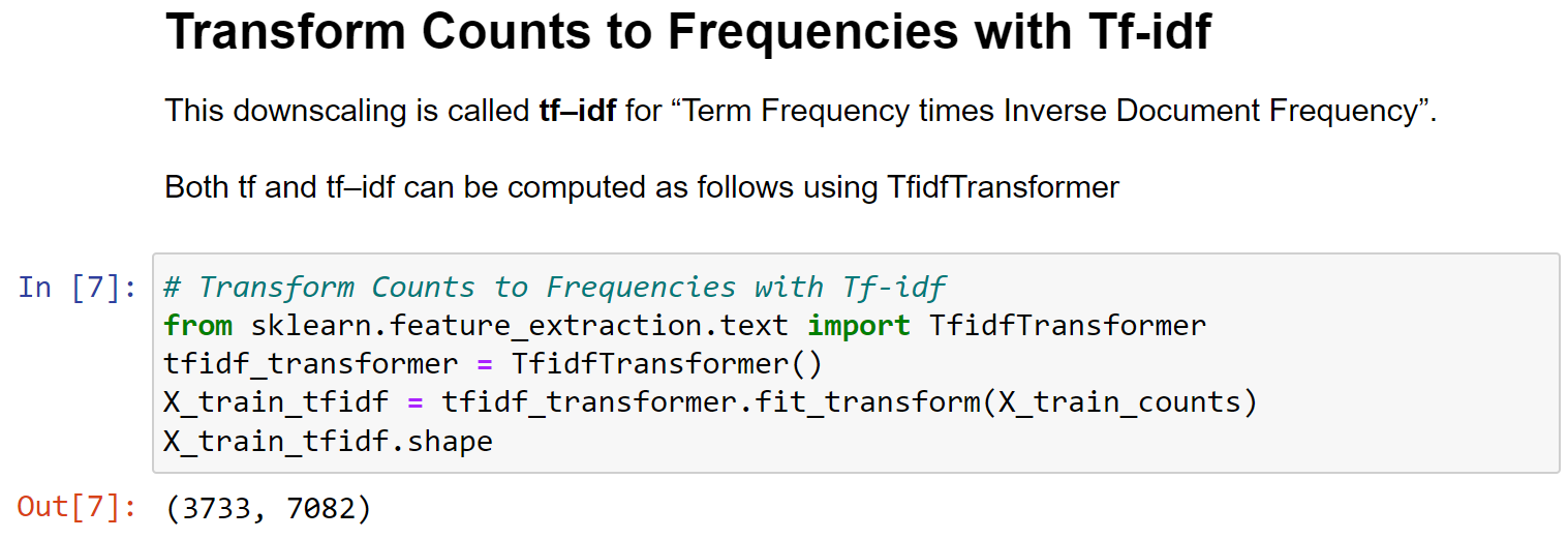
5.4 TF-IDF
- TF-IDF = Term Frequency * (1/document Frequency)
- TF-IDF = Term Frequency * Inverse Document Frequency
1 | # Transform Counts to Frequencies with Tf-idf |
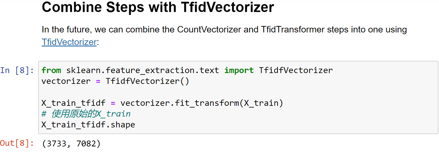
5.5 TF-IDF Vectorizer
- TF-IDF Vectorizer is superior to raw Count Vectorizer
- TF-IDF allows us to understand the context of words across an entire corpus of documents, instead of just its relative importance in a single document
- Scikit-Learn’s
TfidfVectorizerto train and fit our models
1 | from sklearn.feature_extraction.text import TfidfVectorizer |
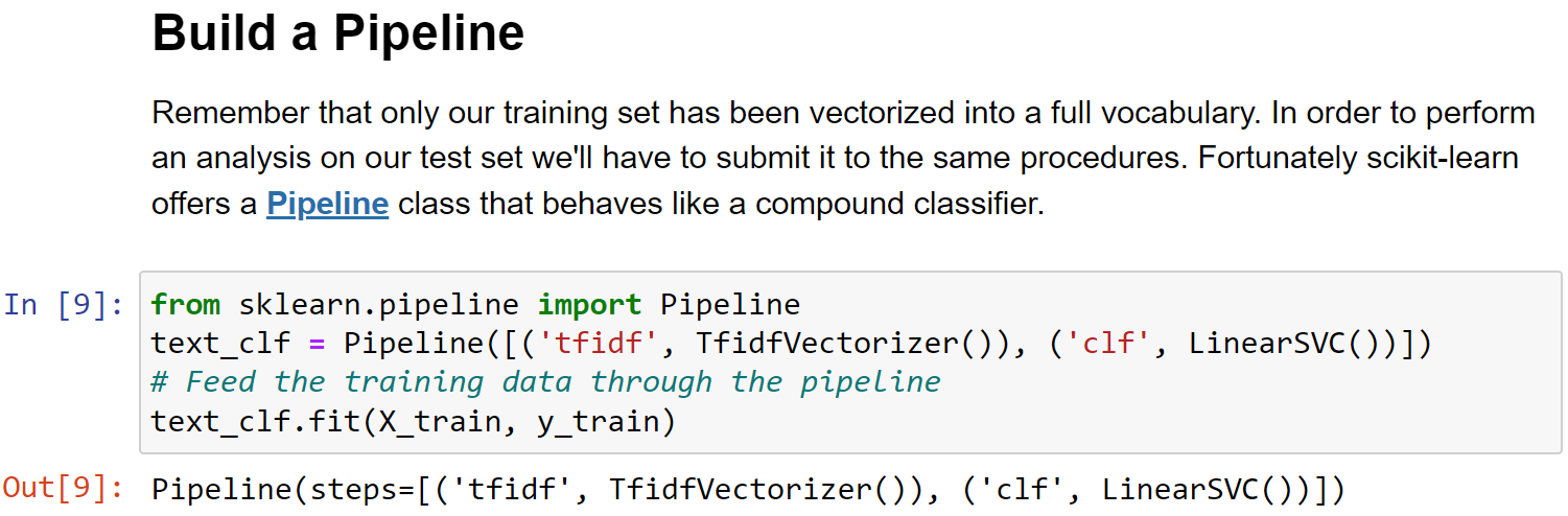
5.6 Pipline
- Pipeline of transforms with a final estimator.
- Sequentially apply a list of transforms and a final estimator. Intermediate steps of the pipeline must be ‘transforms’, that is, they must implement
fitandtransformmethods. The final estimator only needs to implementfit. The transformers in the pipeline can be cached usingmemoryargument. - The purpose of the pipeline is to assemble several steps that can be cross-validated together while setting different parameters. For this, it enables setting parameters of the various steps using their names and the parameter name separated by a
'__', as in the example below. A step’s estimator may be replaced entirely by setting the parameter with its name to another estimator, or a transformer removed by setting it to'passthrough'orNone.
1 | from sklearn.pipeline import Pipeline |
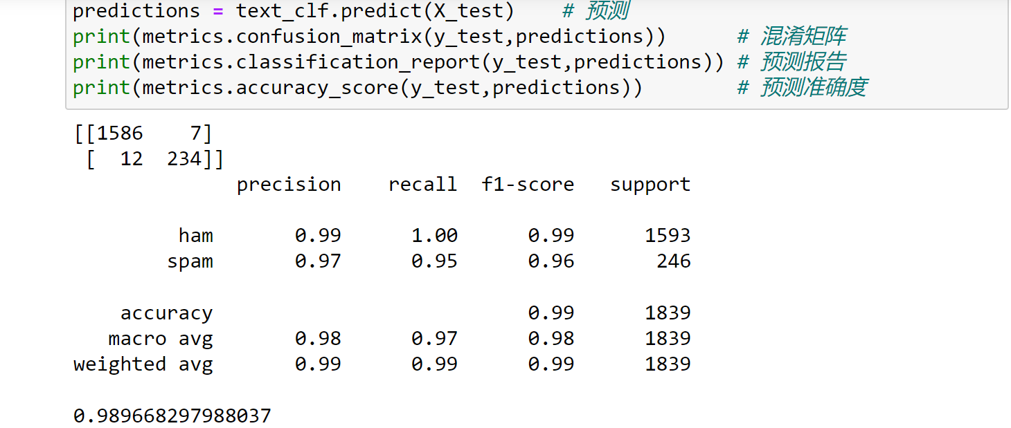
对预测结果进行评估验证,可以发现此时准确度有明显的提升:
1 | from sklearn import metrics |
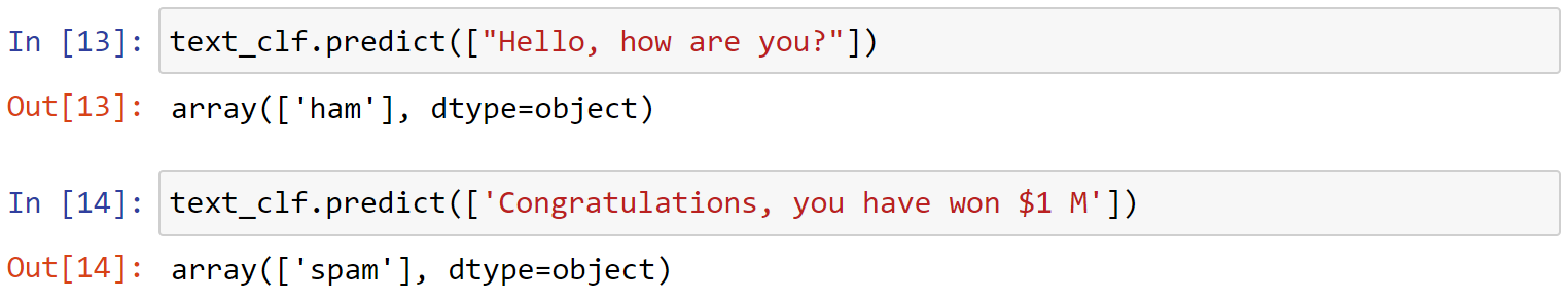
使用该算法预测两个句子:
1 | text_clf.predict(["Hello, how are you?"]) |
Text Classification Project:
- Read in a collection of documents - a corpus
- Transform text into numerical vector data using a pipeline
- Create a classifier
- Fit/train the classifier
- Test the classifier on new data
- Evaluate performance
6. Semantic Analysis
6.1 概述
- Semantic analysis is the process of drawing meaning from natural language text
- It attempts to mimic the process humans follow, i.e., processing words in the context of their appearance, relating them with other words, and selecting most appropriate meaning (removing ambiguities)
- Context plays an important role, it helps to attribute the correct meaning
- It is an essential sub-task of NLP and the driving force behind machine learning tools such as chatbots, search engines and text analysis
How does Semantic Analysis work?
- Semantic analysis begins by understanding relationships between lexical items (words, phrasal verbs, noun phrases, etc.)
- It creates lexical hierarchies using:
- Hyponyms/Hypernyms-inheritance like structure
- Meronomy-whole/part like structure
- Polysemy-relationship based on common core meaning
- Synonyms-words with same meaning and can substitute
- Antonyms-words with opposite meaning
- Homonyms-words with similar sound & spelling but different meaning
- Semantic analysis considers signs and symbols (semiotics) and collocations (words that often go together)
- Automated semantic analysis works with the help of machine learning algorithms. By feeding semantically enhanced algorithms with sample text,you can train machines to make accurate predictions based on past observations
- Two important sub-tasks involved in this approach are:
- Word sense disambiguation (e.g.,Orange could mean color,fruit, or a county in California)
- Relationship extraction(e.g.,relationship between persons, organizations, and places)
6.2 Semantic Analysis Techniques
Classification Models
- Topic Classification:Sorting text to predefined topics that they belong to. For example, a service ticket could be regarding a “payment issue” or “shipping problem”.
- Sentiment Analysis:Detecting positive, negative, or neutral emotions. This could mean, for example, how customers feel about a product or service.
- Intent Classification:Classifying text based on what customers intend to do next. This could mean, for example, that customer wants to talk to an expert.
Extraction Models
Keyword Extraction
- Finding relevant words and expressions in a text
- Used for more granular insight,e.g.,a feedback classified as negative, what words or topics are mentioned most often
Entity Extraction
- Identifying named entities in text. This could be customized to automatically detect company specific texts, e.g.,product/service names, ticket # etc.
7. Word Vectors
What are word vectors?
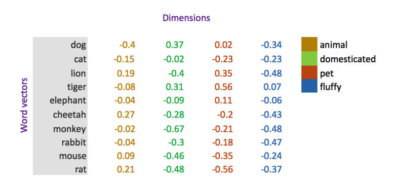
- A word vector is a set of numbers that represent the meaning of a word,with a lot of contextual information
- A vector representing a word is an array of real-valued numbers, where each point captures a dimension of word’s meaning
- These numbers encode the meaning of words in such a way that words close in vector space are expected to have similar meaning
- Creation of word vectors is a critical component of semantic analysis, and this approach is called word embedding
Why word vectors?
- Representing words with numbers enables mathematical operations: such as detecting (cosine) similarity, adding &subtracting vectors, finding associations, and predicting meaning
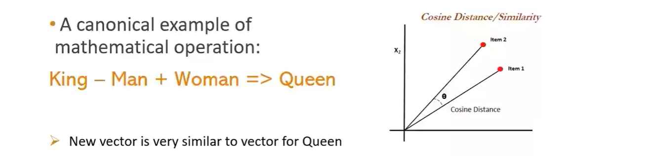
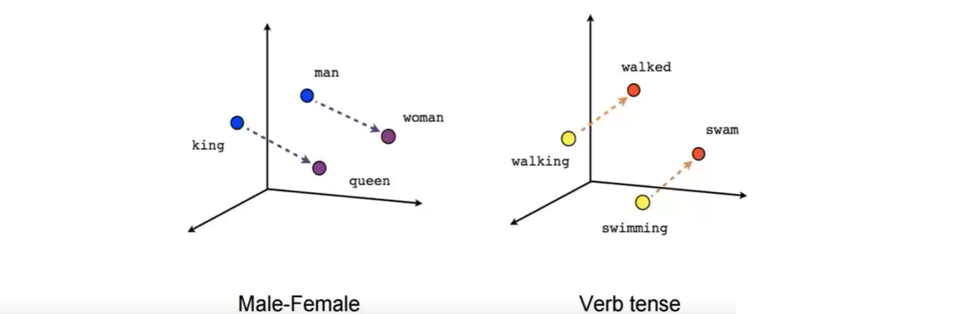
Interesting relationships can be established between word vectors.
How are word vectors created?
- Word vectors are created by feeding a large corpus of text into a deep learning model (neural network)
- Word vectors are created by following distributional hypothesis, which states-“You shall know a word by the company it keeps”
- Words that share similar context tend to have similar meaning.
- Models either use context to predict a target word (CBOW method) or use a word to predict a target context (Skip-Gram method)
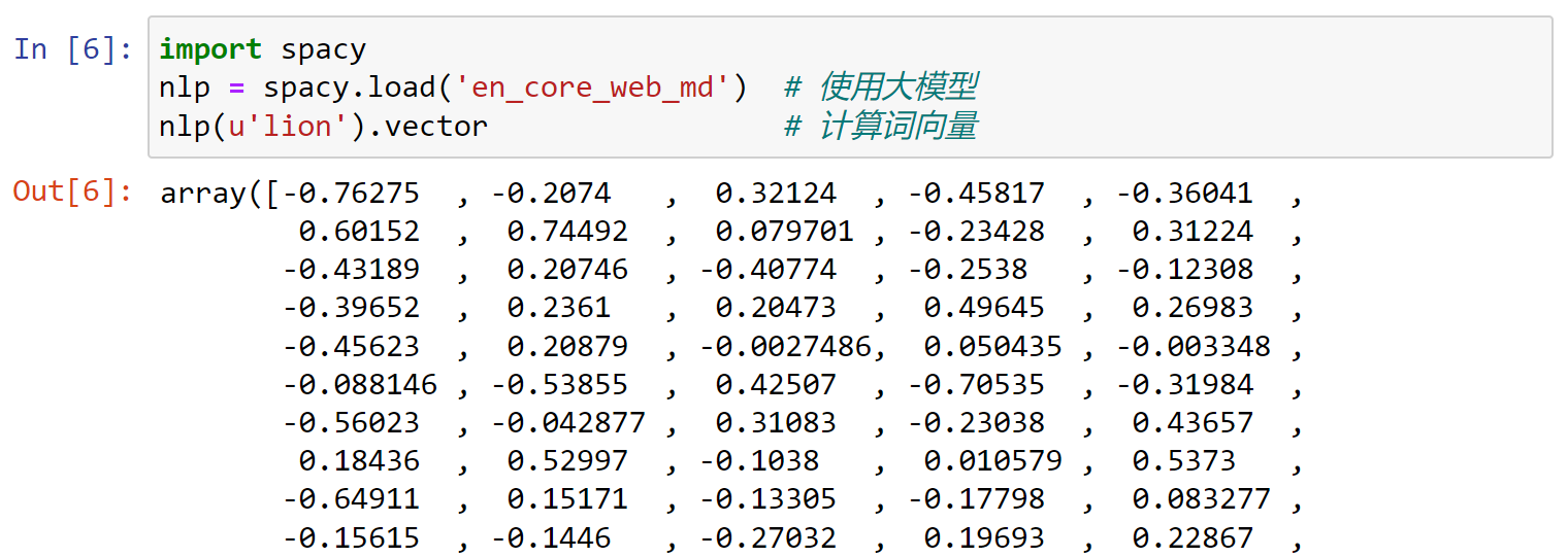
word2vecis a two-layer neural network model
1 | import spacy |
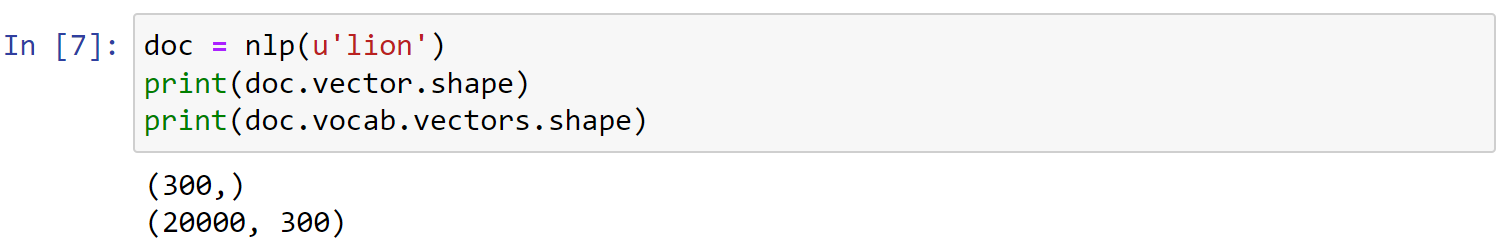
查看向量的维度:
1 | doc = nlp(u'lion') |
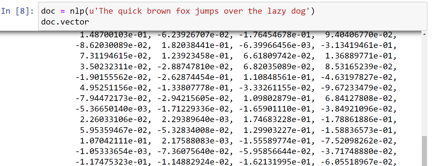
查看句子的向量表示,同样是300个维度:
1 | doc = nlp(u'The quick brown fox jumps over the lazy dog') |
Identifying similar vectors:The best way to expose vector relationships is through the .similarity() method of Doc tokens.
1 | tokens = nlp(u'dog cat monkey') |
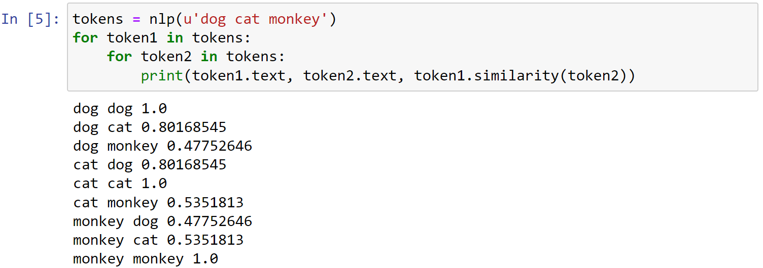
Note that order doesn’t matter. token1.similarity(token2) has the same value as token2.similarity(token1)
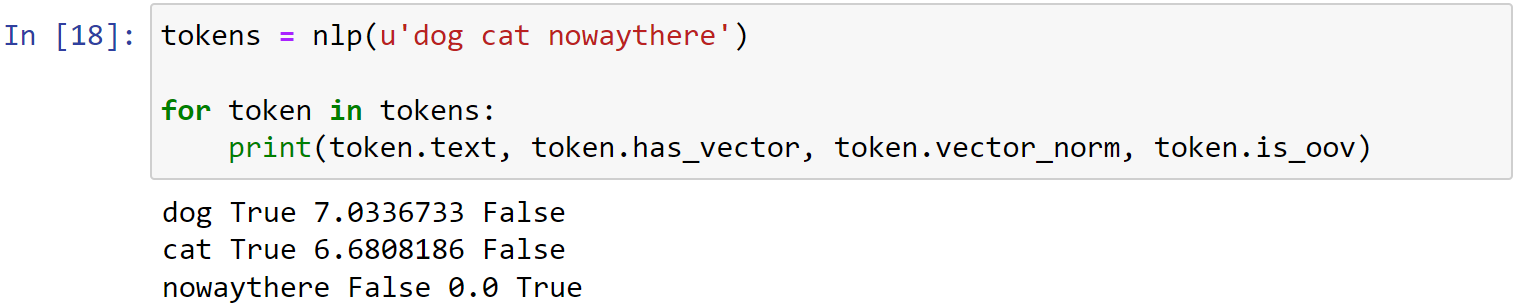
Vector norms
It’s sometimes helpful to aggregate 300 dimensions into a Euclidian (L2) norm, computed as the square root of the sum-of-squared-vectors. This is accessible as the .vector_norm token attribute. Other helpful attributes include .has_vector and .is_oov or out of vocabulary.
1 | tokens = nlp(u'dog cat nowaythere') |
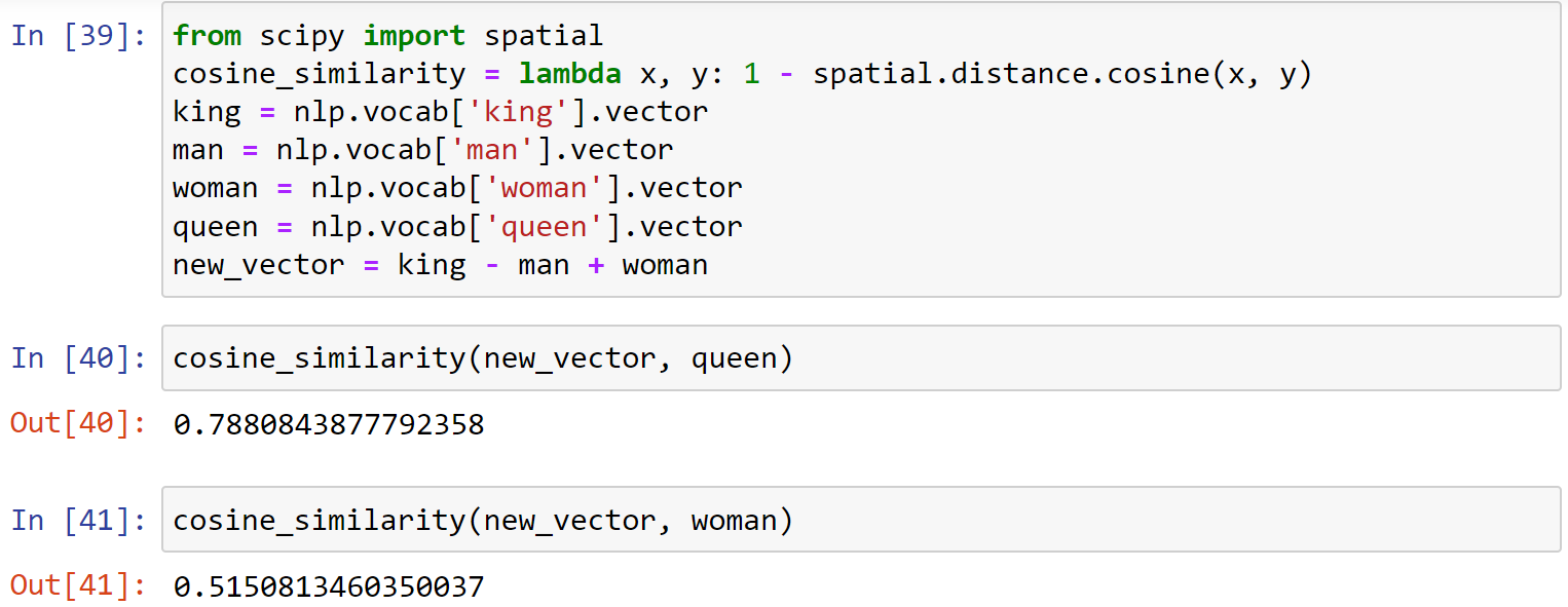
Vector arithmetic
Believe it or not, we can actually calculate new vectors by adding & subtracting related vectors. A famous example suggests
"king" - "man" + "woman" = "queen"
1 | from scipy import spatial |
8. sentiment analysis
What is sentiment analysis?
- Sentiment analysis is a method that detects polarity (e.g.,positive or negative opinion) within the text
- It is also used to detect emotions (happy, sad, angry, etc.), urgency (urgent vs. not urgent) and intentions (interested vs. not interested)
- Sentiment analysis can be rule-based (manually crafted rules), automatic(feature extraction & text classification),or hybrid
- Sentiment analysis is hard due to multiple reasons - sarcasm, idioms, negation handling, adverbial modifiers, comparisons etc.
How is sentiment analysis used?
- Since people share their opinion more openly than ever before, sentiment analysis is useful in a variety of ways such as: social media monitoring, customer support, customer feedback, brand monitoring, voice of customer, market research, etc.
- Sentiment analysis can also be used as a real-time analysis tool, especially if events requiring urgent action need to be detected
9. VADER
- Valence Aware Dictionary for Sentiment Reasoning (VADER) is a model used for text sentiment analysis that is sensitive to both polarity (positive/negative) and intensity (strength) of emotion
- Primarily, VADER sentiment analysis relies on a dictionary which maps lexical features to emotion intensities called sentiment scores
- The sentiment score of a text can be obtained by summing up the intensity of each word in the text
- VADER is a rule-based system
- VADER understands that words like “love”, “like”, “enjoy”,“happy” all convey a positive sentiment.
- VADER is intelligent enough to understand basic context of these words, such as “did not love” as a negative sentiment.
- It uses rules to also understand that the capitalization and punctuation enhance intensity of emotions, e.g., “LOVE!!!!”
- VADER is available in the NLTK package and can be applied directly to unlabeled data.
Download the VADER lexicon.
1 | import nltk |
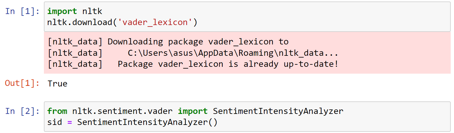
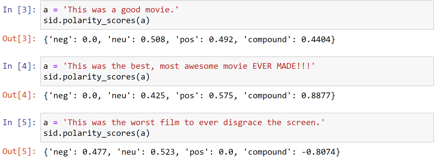
VADER’s SentimentIntensityAnalyzer() takes in a string and returns a dictionary of scores in each of four categories:
- negative
- neutral
- positive
- compound (computed by normalizing the scores above)
计算每个句子中包含的情感比例:
1 | a = 'This was a good movie.' |
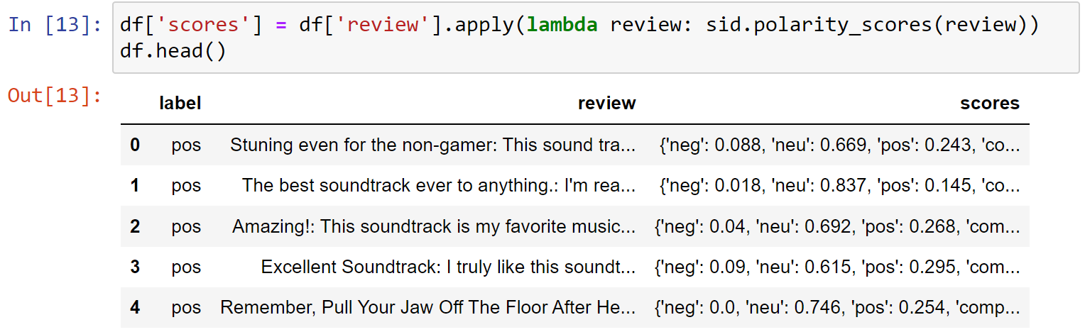
Adding Scores and Labels to the DataFrame
在score后加入一列review数据
1 | df['scores'] = df['review'].apply(lambda review: sid.polarity_scores(review)) |
10. Sentiment Analysis Project
For this project, we’ll perform the same type of NLTK VADER sentiment analysis, this time on our movie reviews dataset.
The 2,000 record IMDb movie review database is accessible through NLTK directly with
1 | from nltk.corpus import movie_reviews |
However, since we already have it in a tab-delimited file we’ll use that instead.
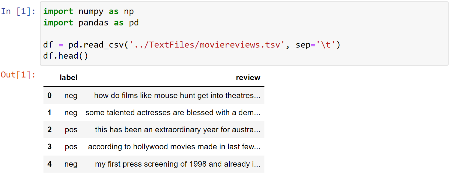
Load the Data
1 | import numpy as np |
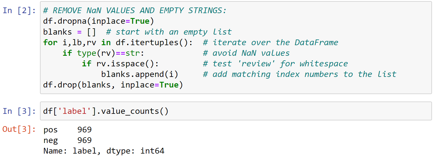
Remove Blank Records (optional)
1 | # REMOVE NaN VALUES AND EMPTY STRINGS: |
Import SentimentIntensityAnalyzer and create an sid object
1 | from nltk.sentiment.vader import SentimentIntensityAnalyzer |
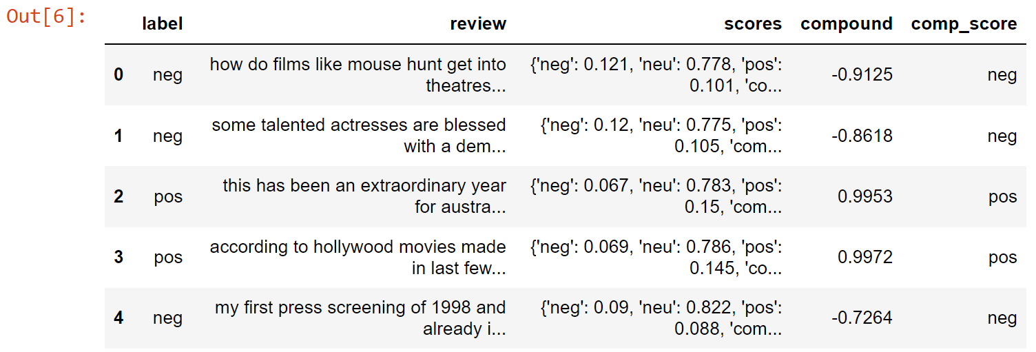
Use sid to append a comp_score to the dataset
1 | df['scores'] = df['review'].apply(lambda review: sid.polarity_scores(review)) |
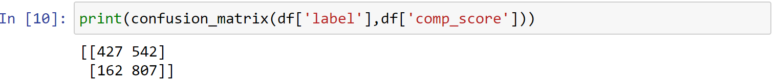
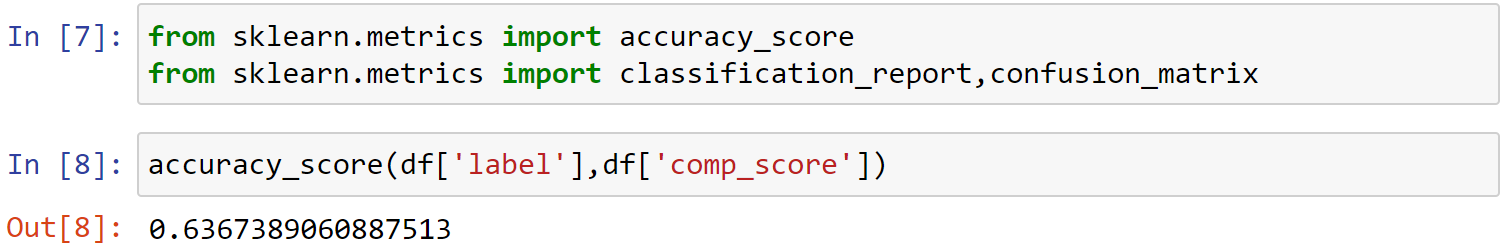
Perform a comparison analysis between the original label and comp_score
1 | from sklearn.metrics import accuracy_score |
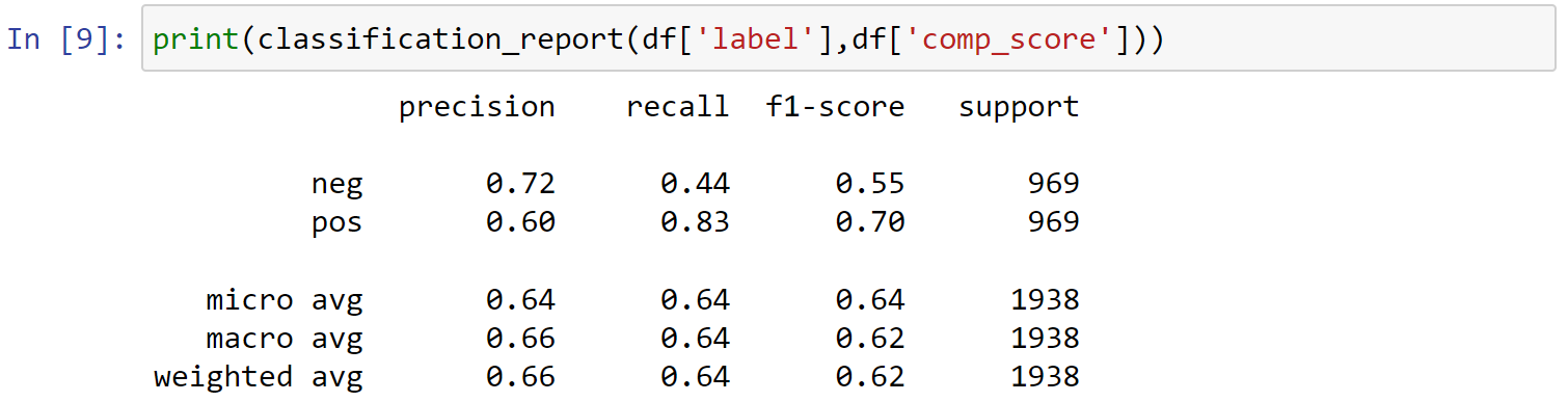
1 | print(classification_report(df['label'],df['comp_score'])) |
1 | print(confusion_matrix(df['label'],df['comp_score'])) |